1. Introduction: What Is Synthetic Aperture Radar (SAR)?

Synthetic Aperture Radar (SAR) is an active remote sensing technology that transmits microwave pulses toward Earth’s surface and records the energy scattered back to the satellite. By processing these radar echoes, SAR systems produce images that reveal information about surface roughness, moisture, vegetation, buildings, and water.

Unlike conventional optical satellites, which measure reflected sunlight, SAR instruments generate their own illumination. This fundamental difference makes radar satellite remote sensing particularly valuable when optical imagery is unavailable because of clouds, darkness, or poor lighting.

For example, optical sensors such as Sentinel-2 may struggle to capture a clear image during heavy cloud cover. Sentinel-1 can generally acquire useful imagery in the same conditions because its C-band microwaves are not blocked by ordinary cloud cover in the way visible light is. It also operates during both day and night. Heavy precipitation, surface conditions, and vegetation can still affect radar observations, so SAR is not completely unaffected by weather or environmental conditions.

According to the Copernicus Sentinel-1 mission documentation, Sentinel-1 provides radar observations for applications including flood monitoring, land mapping, coastal observation, and disaster management. Implementing a complete SAR Synthetic Aperture Radar Sentinel 1 GIS workflow requires several specific preprocessing steps to get analysis-ready data.

Why use Sentinel-1 in GIS?

Sentinel-1 is useful for GIS and remote sensing students because its data are freely available through the Copernicus Data Space Ecosystem and can be processed with open-source software such as ESA SNAP and QGIS.

Common applications include:

• Flood mapping: Detecting changes in surface water extent after heavy rainfall or river overflow.
• Agricultural monitoring: Observing changes in crop structure, field moisture, and vegetation.
• Forest monitoring: Investigating vegetation structure and changes in forest cover.
• Urban analysis: Studying built-up areas and radar scattering patterns.
• Coastal monitoring: Mapping shorelines and changes in exposed water surfaces.

This guide focuses on processing Sentinel-1 Ground Range Detected (GRD) data and using it to identify potential surface-water and flood-inundation areas.

2. Core Concepts for Beginners

Before downloading radar imagery, understand three key ideas: wavelength, polarization, and backscatter.

2.1 Wavelengths and radar bands

Radar systems operate at different microwave frequencies. Their wavelengths influence how the radar interacts with objects on Earth’s surface.

Radar band	Approximate wavelength	Typical applications
X-band	2.5–3.8 cm	Detailed surface mapping, infrastructure, and high-resolution observation
C-band	5–6 cm	Flood monitoring, agriculture, and land-cover change
L-band	15–30 cm	Forest structure, biomass studies, and some soil-surface investigations

Sentinel-1 uses C-band radar, with a wavelength of approximately 5.6 cm. Its response depends on factors such as surface roughness, moisture, vegetation structure, and the viewing geometry.

Longer wavelengths, such as L-band, can interact with larger vegetation structures and may penetrate certain vegetation canopies more effectively than C-band. However, penetration depends on vegetation density, moisture, wavelength, and other conditions. Radar does not simply see through every object.

2.2 Polarization modes: VV, VH, HH, and HV

Polarization describes the orientation of the electromagnetic wave when it is transmitted and received.

The two letters in a polarization label represent the transmitted and received orientations:

Polarization	Meaning	General interpretation
VV	Vertical transmit, vertical receive	Co-polarized return; useful for open-water and land-surface analysis
VH	Vertical transmit, horizontal receive	Cross-polarized return; often useful for studying vegetation and structural scattering
HH	Horizontal transmit, horizontal receive	Co-polarized return used by radar systems configured for horizontal transmission
HV	Horizontal transmit, vertical receive	Cross-polarized return, often useful for vegetation-structure studies

Important: Sentinel-1 does not record all four combinations in every acquisition. For land applications, you will commonly encounter dual-polarization products containing VV and VH. Other acquisition configurations may provide different polarization combinations.

The usefulness of each polarization depends on the study. VV can be effective for detecting changes in open-water areas, while VH offers complementary information about vegetation and scattering. Neither is universally superior for every flood or land-cover application.

2.3 Understanding radar backscatter

Backscatter is the portion of radar energy scattered back toward the sensor. Its intensity is influenced by surface roughness, moisture, geometry, material properties, and polarization.

Consider how radar interacts with three surface types:

• Smooth, open water: Often produces low backscatter because most radar energy reflects away from the satellite.
• Rough ground: Can scatter more energy back toward the sensor, producing higher backscatter.
• Buildings and vegetation: Can produce complex responses through surface, volume, and double-bounce scattering.

Radar images are often displayed using decibels (dB). Lower, more negative dB values generally indicate weaker backscatter, while higher values indicate stronger backscatter.

This explains why open water may appear dark in a Sentinel-1 image. However, wind-roughened water, flooded vegetation, and urban flooding can produce different patterns, so darkness alone is not definitive proof of flooding.

3. Step-by-Step Sentinel-1 Processing Workflow

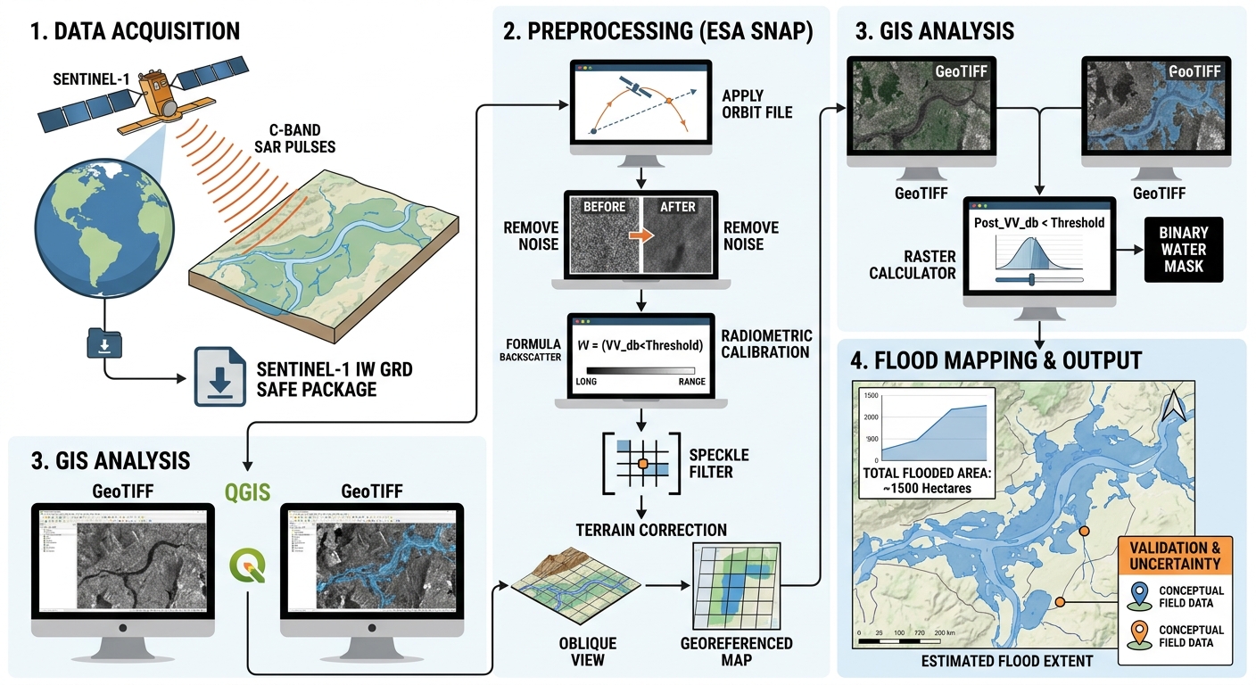
The recommended beginner workflow uses Sentinel-1 GRD imagery, ESA SNAP for radar preprocessing, and QGIS or ArcGIS Pro for GIS analysis.

Step 1: Download Sentinel-1 GRD data

Begin by accessing the Copernicus Data Space Browser.

1. Create an account and open the browser.

Register for a free account, sign in, and navigate to the geographical area you want to study.

2. Define your area of interest (AOI).

Search for a study location or draw a polygon around it. For your first project, choose a river floodplain, lake shoreline, or relatively flat agricultural area.

3. Choose a date range.

For flood mapping, ideally identify two acquisitions:

• A pre-flood image, captured before the flooding event.
• A post-flood image, captured during or shortly after the event.

Choose images with comparable acquisition conditions. The same relative orbit and ascending or descending pass direction are important because differences in viewing geometry can cause apparent changes unrelated to flooding.

4. Filter for Sentinel-1 products.

Select Sentinel-1 and choose a GRD (Ground Range Detected) product. For many land applications, Interferometric Wide Swath (IW) mode with VV and VH polarization is a practical starting point.

GRD data contain detected radar intensity and do not retain the original phase information. They are suitable for many intensity-based applications, including flood mapping, but are not a replacement for Single Look Complex (SLC) data when phase-based analysis such as interferometry is required.

5. Download the product.

Select a suitable result and download the product. Depending on the available product format, you may receive a compressed SAFE package or another supported format. Keep the original download unchanged and extract the archive if necessary.

The Copernicus Sentinel-1 data documentation explains the available product types and formats.

Output: A Sentinel-1 GRD product ready for preprocessing.

Step 2: Preprocess Sentinel-1 data in ESA SNAP

Raw or minimally processed radar imagery should not be treated as a finished analysis layer. Preprocessing corrects systematic errors, produces meaningful backscatter values, and improves geographic alignment.

Download SNAP and its Sentinel-1 Toolbox from the ESA STEP website.

Open SNAP and load the downloaded Sentinel-1 product.

2.1 Apply orbit file

Open the Apply Orbit File operator, generally available under the Radar menu.

Orbit information improves knowledge of the satellite’s position during acquisition, supporting accurate geolocation.

Select the appropriate orbit-file option available in SNAP, retain the suitable default settings for an introductory workflow, and run the operator.

2.2 Remove thermal and border noise

Radar imagery may contain unwanted thermal noise and low-quality border pixels.

Where applicable to the product, use SNAP’s Thermal Noise Removal and Remove-GRD-Border-Noise operators. Follow the product documentation and processing history to avoid applying a correction twice when it has already been performed.

These steps help reduce unwanted signals that could otherwise be mistaken for land or water features.

2.3 Perform radiometric calibration

Calibration converts image measurements into meaningful radar backscatter coefficients.

Open Calibration and select the polarization bands required for your analysis. For a typical flood-mapping exercise, select the available VV and VH bands and calibrate to Sigma nought (σ⁰).

Sigma nought is a commonly used measure of radar backscatter normalized to the reference area and viewing geometry. Other coefficients, such as Gamma nought (γ⁰), may be appropriate for particular applications and terrain treatments.

Avoid using uncalibrated digital numbers as though they were directly comparable physical backscatter measurements.

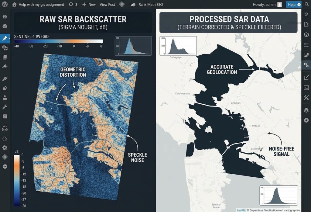
2.4 Apply speckle filtering

Speckle is the granular appearance commonly found in coherent radar imagery. It results from interference among radar returns from many scatterers within a resolution cell.

In SNAP, use the Speckle-Filter operator if smoothing is appropriate for your study. A Lee-family filter, such as Refined Lee where supported by the input product and workflow, is one possible choice.

Begin with a modest filter window, such as 3 × 3, and assess the result before increasing the window size.

Speckle filtering is optional rather than universally mandatory. Strong filtering can erase narrow rivers, small flooded fields, and other features that matter to the analysis. For common GRD workflows, filtering before terrain correction is a useful starting point because resampling during geocorrection can further alter the image texture.

2.5 Perform terrain correction

Radar images are acquired from an oblique viewing angle, so their original image coordinates do not directly correspond to a standard map grid.

Open Range-Doppler Terrain Correction and configure:

• Digital Elevation Model (DEM): Select an appropriate DEM, such as Copernicus DEM or SRTM, where available and suitable for your location.
• Target coordinate reference system: Choose a suitable projected CRS, such as the appropriate UTM zone for your study area.
• Pixel spacing: Select a suitable output spacing, often 10 m or 20 m for a Sentinel-1 GRD exercise.
• Resampling: Use an appropriate method, such as bilinear interpolation for continuous backscatter data.

Run the operator and verify that the resulting image aligns correctly with geographic reference layers.

Terrain correction improves geographic positioning, but it does not recover information lost through radar shadow or other acquisition-related distortions. In hilly terrain, radiometric terrain flattening may also be needed to address slope-related brightness differences.

2.6 Convert calibrated backscatter to decibels

For threshold-based water extraction, a dB representation is often convenient.

Use SNAP’s LinearToFromdB operator to convert the calibrated linear backscatter output to dB, following the appropriate processing sequence for your study.

For power measurements, the conversion is:

[
\sigma^0_{\mathrm{dB}}=10\log_{10}(\sigma^0)
]

The conversion requires positive linear power values. Handle zero, invalid, and NoData pixels carefully so that logarithms do not introduce infinite or misleading values.

Finally, inspect the calibrated VV and VH layers visually. Open water often appears dark, while land surfaces frequently show stronger or more variable returns.

Output: Georeferenced, calibrated VV and VH backscatter rasters ready for GIS analysis.

Step 3: Import processed SAR rasters into QGIS or ArcGIS Pro

Export your processed backscatter bands from SNAP in a GIS-compatible format, such as GeoTIFF.

In SNAP, use the available export or product-band export options to save the required bands. Confirm that the selected output is the processed raster, rather than the original uncorrected measurement.

In QGIS

1. Open QGIS and create a new project.
2. Select Layer → Add Layer → Add Raster Layer.
3. Browse to the exported VV or VH GeoTIFF and add it to the map.
4. Open Layer Properties → Symbology and choose a single-band grayscale renderer.
5. Adjust the display range so differences in backscatter intensity are visible.
6. Add a boundary, river network, or existing water-body dataset to help interpret the image.

Use the Processing Toolbox and Raster Calculator for threshold-based classification.

In ArcGIS Pro

1. Create a project and add the processed GeoTIFF using Map → Add Data.
2. Inspect the raster in the Contents pane and adjust its symbology.
3. Check the coordinate reference system and spatial alignment against your other layers.
4. Use Raster Calculator or an appropriate raster conditional tool to create a water-candidate layer.

The Esri Sentinel-1 SAR processing tutorial provides an additional workflow reference for users of ArcGIS Pro.

Practical note: Sentinel-1 IW GRD products may have approximately 10 m pixel spacing in common outputs, but this does not mean every feature is resolved at a true 10 m spatial resolution. Pixel spacing and effective spatial resolution are different concepts.

Step 4: Extract surface water and flood inundation extent

Once your processed SAR rasters are in GIS, you can create an initial water mask using backscatter thresholds.

4.1 Identify potential water pixels

Open water frequently exhibits low backscatter because a relatively smooth water surface reflects much of the incoming radar energy away from the satellite.

For an introductory exercise, suppose visual inspection and reference information suggest that a threshold of −17 dB is a reasonable starting point for the VV image.

This value is illustrative only. It is not a universal Sentinel-1 flood-mapping threshold. The appropriate threshold varies with the location, polarization, acquisition, surface conditions, calibration, and processing workflow.

In the QGIS Raster Calculator, an example expression is:

"VV_db@1" < -17

Replace VV_db@1 with the actual name of your calibrated dB raster.

The resulting binary raster identifies pixels below the example threshold. A value of 1 represents a potential-water candidate, while 0 represents a pixel that does not meet the condition.

For ArcGIS Pro, a corresponding conditional expression is:

Con("VV_db" < -17, 1, 0)

Replace the layer name with your actual raster name and confirm how NoData is handled.

4.2 Compare pre-flood and post-flood imagery

A low-backscatter water mask shows potential water, not necessarily new floodwater. Rivers and lakes that existed before a flood can also produce low returns.

To identify possible newly inundated areas, classify both dates using a consistent method:

1. Create a water-candidate mask for the pre-flood image.
2. Create a water-candidate mask for the post-flood image.
3. Compare the two masks.
4. Retain pixels that meet the post-flood water condition but did not meet the pre-flood water condition.

Conceptually:

[
\text{New water}=\text{Post-flood water}\cap\text{Not pre-flood water}
]

For the simplified threshold example, the logic can be represented as:

("Post_VV_db@1" < -17) AND
("Pre_VV_db@1" >= -17)

This expression assumes the input rasters are aligned, use comparable processing, and have appropriate NoData handling. It identifies pixels that cross the chosen threshold; it does not independently prove that they were flooded.

Use a suitable permanent-water mask, historic imagery, land-cover data, and visual interpretation to reduce false positives. For more reliable results, consider adaptive thresholds, multitemporal analysis, or validated flood-mapping methods.

4.3 Validate the flood extent

Inspect the result against rivers, lakes, elevation, and known flood observations.

Potential problems include:

• Smooth roads and bare ground being classified as water.
• Shadows and low-return areas creating false water candidates.
• Flooded vegetation remaining bright because of complex scattering.
• Urban flooding producing stronger radar returns from building-water interactions.
• Water levels changing naturally between acquisition dates.

When suitable reference data are available, compare the flood mask with field observations, high-resolution imagery, official flood information, or another independent dataset.

4.4 Calculate the flooded area

After refining the result, calculate the area of mapped flood pixels using a projected coordinate system with appropriate linear units.

For a raster with square 10 m pixels, each valid pixel represents a nominal grid-cell area of 100 m². Multiply the count of selected flood pixels by the grid-cell area, then convert the result to hectares or square kilometres as required.

Report the result as an estimated mapped inundation area, and document the threshold, dates, CRS, pixel spacing, masks, and validation method.

4. Common Challenges in SAR Synthetic Aperture Radar Sentinel 1 GIS Workflows

Speckle noise

Speckle can make classification results look fragmented and create isolated water candidates.

How to address it: Test a modest speckle filter and compare the image before and after filtering. Use temporal averaging when suitable images are available, and avoid smoothing that removes narrow water features.

Layover and foreshortening

Mountainous terrain introduces geometric distortions because radar observes the surface from the side rather than directly overhead.

• Foreshortening: Slopes facing the radar appear compressed.
• Layover: Returns from elevated parts of a slope may arrive before returns from lower parts, causing features to appear displaced or inverted.
• Radar shadow: Terrain blocks the radar beam, resulting in little or no return behind an obstruction.

How to address them: Use a suitable DEM, correct the image geometrically, inspect the acquisition direction, and exclude areas affected by severe distortion where appropriate. Radiometric terrain correction can help improve slope-related backscatter comparisons, but terrain correction cannot restore features hidden by radar shadow.

Choosing the wrong threshold

A single backscatter threshold can perform poorly across different land covers or acquisition conditions.

How to address it: Examine VV and VH separately, use the image histogram as supporting evidence, compare pre-flood and post-flood imagery, and test candidate thresholds against reference information. Document any selected values so another analyst can reproduce the workflow.

Comparing incompatible images

Differences in orbit direction, incidence geometry, season, or surface moisture may appear as land-cover changes.

How to address it: Prefer acquisitions from the same relative orbit and pass direction when possible. Keep the processing settings and target grid consistent and investigate whether observed differences are caused by flooding or unrelated surface changes.

5. Conclusion

SAR Synthetic Aperture Radar Sentinel 1 GIS workflows allow remote sensing students to investigate Earth’s surface when optical imagery is restricted by clouds or darkness. By understanding C-band radar, polarization, and backscatter, beginners can interpret Sentinel-1 imagery more confidently.

The essential workflow is to download Sentinel-1 GRD data from Copernicus Data Space, apply suitable corrections in SNAP, export calibrated rasters, and analyse them in QGIS or ArcGIS Pro. For flood mapping, combining a carefully selected backscatter threshold with pre-flood imagery, permanent-water information, terrain checks, and validation produces more defensible results than classifying dark pixels alone.

Remember that a SAR-derived water mask is an estimate, not automatic proof of flooding. Good results depend on suitable data, reproducible processing, an understanding of radar limitations, and independent validation. Mastering SAR Synthetic Aperture Radar Sentinel 1 GIS processing provides a robust alternative to optical imagery for many GIS applications.

6. Resources for Further Learning

1. Copernicus Data Space Browser — Search for, inspect, and download Sentinel imagery.
2. Copernicus Sentinel-1 Documentation — Learn about Sentinel-1 product types and data characteristics.
3. ESA SNAP Sentinel-1 Toolbox — Access radar processing tools and documentation.
4. ESA SNAP Online Help — Review operators for calibration, speckle filtering, thermal-noise removal, and terrain correction.
5. Esri: Process Sentinel-1 SAR Data — Follow an ArcGIS Pro SAR preprocessing workflow.
6. NASA SAR Handbook — Study the principles and applications of spaceborne synthetic aperture radar.
7. Space4Water: Flood Mapping with Sentinel-1 SAR — Explore a practical flood-mapping methodology.