Table of Contents

Standard Deviational Ellipse & Mean Center Analysis: Mapping Spatial Directional Trends

1. Introduction: Why Analyze Spatial Distribution?

Imagine you have collected 5,000 wildlife sightings, mapped thousands of disease cases, or recorded customer locations for a chain of retail stores. A point map shows where the observations occur, but it may not immediately reveal the overall geographic pattern.

Are the observations concentrated around one location? Do they extend farther in a particular direction? Has the geographic center shifted over time?

Spatial distribution statistics help answer these questions by summarizing the location, spread, and orientation of geographic features.

Two useful methods are Mean Center and the Standard Deviational Ellipse (SDE). Together, they provide a compact description of a spatial distribution that can be compared across regions, time periods, or groups.

The methods are available through the Measuring Geographic Distributions tools in ArcGIS Pro. QGIS users can calculate mean coordinates using built-in processing tools and use plugins for standard deviational ellipses and other spatial statistics.

This tutorial explains the concepts and guides you through preparing point data, calculating geographic centers, creating ellipses, and comparing spatial patterns across multiple years. Utilizing a Standard Deviational Ellipse Mean Center GIS workflow helps analysts uncover hidden geographic patterns.

2. Core Concepts Explained

2.1 Mean Center: Finding the average geographic location

The Mean Center is the average X and Y coordinate of a set of spatial features. It provides a single point representing the geographic center of their distribution.

For example, if you map the locations of 100 public hospitals, the mean center indicates the average geographic location of those hospitals.

The mean center is calculated from the coordinate values, not by identifying the most frequently occupied location. It might fall in a park, a river, or an unoccupied area because its purpose is to summarize the distribution rather than identify an actual feature. When calculating coordinates in a Standard Deviational Ellipse Mean Center GIS setup, weight fields can adjust point influence.

The mean center is useful for:

Summarizing the geographic concentration of retail stores.
Comparing the average location of wildlife observations.
Tracking changes in the distribution of disease cases.
Measuring shifts in settlement or infrastructure patterns over time.

A weighted mean center gives more influence to features with larger values in a selected numeric field. For example, store locations could be weighted by customer counts, or wildlife locations by a meaningful measure of activity.

Use weights only when they represent a defensible measure of importance. Otherwise, calculate an unweighted center.

See Esri’s Mean Center documentation.

2.2 Median Center: A center less affected by outliers

The Median Center identifies the location that minimizes the total Euclidean distance to all observations.

Unlike the mean center, it uses an iterative optimization procedure rather than simply averaging the X and Y coordinates.

This makes the median center less sensitive to extreme observations. For instance, if most wildlife sightings occur within a reserve but a few are recorded far away, those distant locations can pull the mean center toward them. The median center is generally less affected.

Use the median center when you want a geographic center that is more robust to outlying locations.

See the Median Center tool reference.

2.3 Central Feature: Finding an actual feature near the center

The Central Feature tool is related to mean and median center analysis but answers a different question.

Instead of creating a calculated average point, it identifies the actual input feature with the smallest accumulated distance to all other features, based on the selected distance method and any specified weights.

For example, if you have a dataset of retail stores, Central Feature can identify one of the existing stores that is most centrally located relative to the others.

These three tools should not be confused:

Tool	What it identifies	Is the output necessarily an existing input feature?
Mean Center	Average geographic position	No
Median Center	Location minimizing the sum of distances	No
Central Feature	Most centrally located observed feature	Yes

Practical tip: Calculate the mean center and median center together when outliers may influence your results. A large difference between them can indicate an uneven distribution or the presence of distant observations.

2.4 Standard Deviational Ellipse Mean Center GIS: Measuring spread and direction

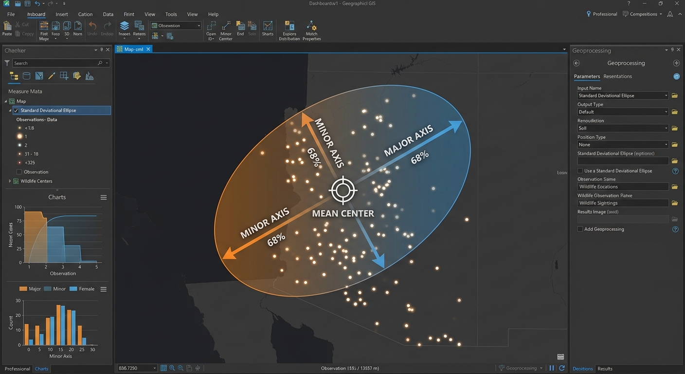
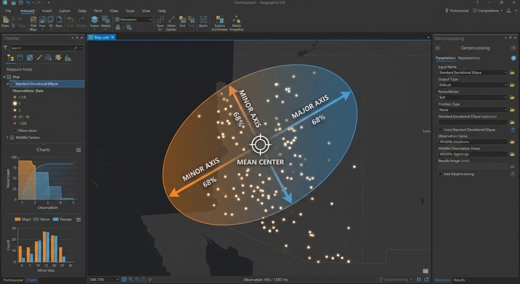
The Standard Deviational Ellipse summarizes the spatial dispersion and orientation of a set of geographic observations.

It produces an ellipse centered on the mean center. The ellipse has:

Major axis: Represents the direction of greatest spread.
Minor axis: Represents the direction of least spread.
Orientation angle: Describes the rotation of the ellipse.
Standard-distance measures: Summarize dispersion along the two principal axes.

Consider two wildlife datasets.

The first contains sightings distributed almost evenly around a central location. Its ellipse is relatively circular, suggesting similar spread in different directions.

The second contains sightings extending along a valley. Its ellipse is elongated, with the major axis aligned approximately with the valley.

The ellipse makes that directional pattern easier to identify than a point map alone.

Important: The major axis describes the direction of greatest spatial dispersion. It does not automatically indicate the direction in which animals travelled, the direction a storm moved, or the direction in which a city expanded over time. Those interpretations require temporal or additional contextual evidence.

3. Understanding 1, 2, and 3 Standard Deviations

In ArcGIS Pro, the Directional Distribution tool lets you create ellipses based on one, two, or three standard deviations.

Ellipse setting	General purpose
1 standard deviation	Summarizes the core spatial distribution
2 standard deviations	Shows a broader extent of dispersion
3 standard deviations	Shows a still broader distribution, potentially including peripheral locations

For data concentrated around a central location and following the spatial distribution assumptions used by the tool, ArcGIS Pro scales its standard deviational ellipses to represent approximately 68%, 95%, and 99% coverage for the respective settings.

These proportions are not guaranteed for every dataset. The underlying distribution, the algorithm used, and the software implementation matter. For example, the QGIS Standard Deviational Ellipse plugin offers alternative calculation methods, some of which use different scaling adjustments.

Do not automatically interpret an SDE as a confidence interval or a guaranteed coverage boundary. It is primarily a descriptive summary of spatial distribution. See How Directional Distribution works and the QGIS Standard Deviational Ellipse plugin documentation.

4. Step 1: Prepare Your Point Dataset

Before calculating a mean center or ellipse, inspect the data carefully. Poor coordinate information or inconsistent sampling can produce misleading spatial summaries.

For this tutorial, consider a wildlife study containing GPS observation points recorded between 2022 and 2025.

The attribute table might contain:

Field	Example	Purpose
`observation_id`	OBS_001	Unique record identifier
`species`	Elephant	Identifies the species
`observation_date`	2024-06-18	Records the observation date
`year`	2024	Supports year-by-year comparison
`weight`	1	Optional weight for the analysis

Each point represents an observation location. If multiple records represent repeated observations of the same animal or event, consider how that sampling structure should affect the analysis.

Data preparation checklist

Confirm that the input layer contains the correct geographic features.
Inspect missing, invalid, or duplicated coordinates.
Check the date or year field if you plan to compare time periods.
Review any outlying observations and verify whether they are genuine.
Decide whether all points should contribute equally or whether a meaningful weight is required.
Ensure that the observation period and sampling method are comparable between groups.

Use an appropriate projected coordinate system

Mean Center and Standard Deviational Ellipse calculate spatial distances and dispersions using coordinate values. For accurate distance-based measurements, use a suitable projected coordinate system for your study area.

A geographic coordinate system such as latitude and longitude expresses positions in angular units, not metres. Calculating standard distances and interpreting them as metres without an appropriate projection can produce misleading results.

In QGIS:

Open Layer Properties → Information and inspect the layer CRS.
Use Export → Save Features As or a suitable reprojection tool to create a version in an appropriate projected CRS.
Check that the output coordinates and units make sense for the region.

In ArcGIS Pro:

Open the layer’s properties and inspect its spatial reference.
Use the Project geoprocessing tool to create a dataset in a suitable projected CRS.
Verify the output coordinate system and map extent.

For large study areas, choose a projection that is appropriate for the geographic extent and analytical purpose.

5. Step 2: Calculate the Mean Center, Median Center, or Central Feature

The next task is to calculate a geographic center that summarizes your observations.

5.1 Run Mean Center in ArcGIS Pro

ArcGIS Pro includes Mean Center, Median Center, and Central Feature in the Spatial Statistics Tools → Measuring Geographic Distributions toolset.

Procedure:

Open Analysis → Tools.
Search for Mean Center.
Select the prepared point layer as the input.
Choose an output feature class and name it Mean_Center.
Select a Weight Field only if you have a suitable numeric field.
Choose a Case Field if you want separate mean centers for groups, such as years or species.
Run the tool.
Add the output point to the map and inspect its location.

If you want a separate center for each year, select a suitable year field as the case field. ArcGIS Pro will calculate a separate mean center for each group.

5.2 Run Median Center in ArcGIS Pro

Open Analysis → Tools.
Search for Median Center.
Select the input feature class.
Choose an output feature class.
Optionally provide a meaningful weight field and case field.
Run the tool.
Compare the output with the mean center.

If the mean and median centers are far apart, inspect the point distribution and outliers before interpreting the difference.

5.3 Run Central Feature in ArcGIS Pro

Open Analysis → Tools.
Search for Central Feature.
Select the input point layer.
Set the distance method to Euclidean or Manhattan, as appropriate.
Specify a weight field if justified.
Choose an output feature class.
Run the tool and inspect the selected feature.

Euclidean distance represents straight-line distance. Manhattan distance measures distance along perpendicular axes, which can be useful for a grid-like layout but is not a substitute for actual road-network distance.

The Central Feature tool identifies a real input feature rather than calculating an entirely new average point. See the Central Feature documentation.

5.4 Calculate mean coordinates in QGIS

QGIS includes a built-in Mean coordinate(s) processing algorithm.

Procedure:

Open the point layer in QGIS.
Open Vector → Analysis Tools → Mean coordinate(s), or search for Mean coordinate(s) in the Processing Toolbox.
Select the input point layer.
Optionally choose a numeric weight field.
Specify a unique ID field if the algorithm requires it.
Leave category grouping blank for one overall center, or select a grouping field to calculate separate centers.
Choose an output layer and run the algorithm.

The resulting point represents the mean coordinates of the input features or the selected groups.

For median center and central feature analysis, QGIS users can explore a compatible plugin such as Spatial Analyzer. Confirm compatibility with your QGIS version before installing and check the method implemented by the plugin.

6. Step 3: Generate the Standard Deviational Ellipse

Once the center has been calculated, create the ellipse that describes the distribution’s dispersion and orientation.

6.1 Generate an ellipse in ArcGIS Pro

ArcGIS Pro provides the Directional Distribution (Standard Deviational Ellipse) tool.

Procedure:

Open Analysis → Tools.
Search for Directional Distribution (Standard Deviational Ellipse).
Select the prepared point dataset as the input.
Specify the output ellipse feature class.
Set Ellipse Size to 1, 2, or 3 standard deviations.
Select a Weight Field if justified by the research objective.
Select a Case Field to generate separate ellipses for groups, such as years.
Run the tool.
Inspect the output polygon and its attributes.

The output ellipse layer contains information describing the mean center, the standard distances along the two axes, and the orientation. When a case field is specified, the tool creates one ellipse for each group that contains eligible observations.

Example: Select year as the case field to create ellipses for 2022, 2023, 2024, and 2025 from the same point dataset.

6.2 Interpret the ellipse attributes

ArcGIS Pro commonly provides fields such as:

CenterX and CenterY: The coordinates of the mean center.
XStdDist and YStdDist: Standard-distance measures along the ellipse axes.
Rotation: The orientation angle for the ellipse.
The case-field value, when the analysis is grouped.

The precise orientation convention should be checked before interpreting or comparing angles between software packages. ArcGIS Pro’s Rotation field represents the long-axis orientation measured clockwise from noon.

The major axis represents the direction of greatest spread, and the minor axis represents the direction of least spread. The ratio of the two axes provides a useful indication of how elongated the distribution is.

An ellipse with a much longer major axis than minor axis suggests a strong directional pattern. An ellipse with similar axes indicates a more isotropic distribution, where the dispersion is relatively similar in different directions.

6.3 Generate an ellipse in QGIS

QGIS does not expose a universally identical native equivalent to ArcGIS Pro’s Directional Distribution tool across all installations, so a common method is to use a compatible plugin.

Procedure using the Standard Deviational Ellipse plugin:

Open Plugins → Manage and Install Plugins.
Search for Standard Deviational Ellipse.
Inspect the plugin information and confirm that it supports your installed QGIS version.
Install and open the plugin.
Select the point layer to analyse.
Choose whether to use all features or only selected features, if supported.
Select a weight attribute when appropriate.
Choose the calculation method available in the plugin.
Run the process and save the resulting ellipse polygon.
Inspect the output attributes, including the mean centre, major and minor standard distances, and orientation.

Plugin algorithms do not always implement the same standard-distance scaling, degrees-of-freedom corrections, or orientation conventions. The QGIS plugin documentation specifically describes differences between its default Yuill approach and the alternative CrimeStat/aspace method. If you need quantitative comparisons between QGIS and ArcGIS outputs, verify that the two tools implement compatible methods.

For advanced reproducible workflows, students can also calculate spatial summaries using Python libraries or custom PyQGIS scripts. Whichever method you choose, record the algorithm, parameters, weight field, projection, and interpretation used.

7. Step 4: Compare Multi-Temporal Ellipses

Comparing spatial distributions across time is particularly useful for studying wildlife migration, urban development, disease patterns, and changes in service use.

For example, suppose your point dataset contains wildlife sightings for four years. You want to determine whether the distribution has shifted eastward and whether its spread has become more elongated.

7.1 Prepare a grouping field

Ensure that your dataset has a year field, such as year.

If the data contain only a date field, derive a year attribute using the field calculator or another suitable processing method.

Before comparison, check:

Each year contains enough observations for meaningful interpretation.
The observation process is reasonably comparable between years.
The same coordinate reference system is used for all analyses.
The same ellipse size and compatible calculation method are used.
The same weight-field logic is applied consistently.

7.2 Generate separate centers and ellipses

In ArcGIS Pro, set the case field to year in the Mean Center and Directional Distribution tools. This produces separate outputs for the groups in a single run.

In QGIS, use a grouping field where the chosen algorithm supports it, or filter the observations by year and run the analysis separately.

7.3 Compare the outputs

Look at three characteristics:

Centre movement: If the mean center shifts east, west, north, or south between years, the average location of observations has changed. The amount and direction of movement can be measured using the projected coordinates of the centers.

Dispersion: If the ellipse becomes larger, the distribution has become more spatially dispersed under the same calculation settings. If it becomes smaller, the observations are more concentrated.

Orientation: If the major axis rotates, the direction of greatest spread has changed. This may indicate a change in the geography of the distribution, but it does not by itself prove a temporal trajectory or causal process.

Comparison	What it may suggest	What it does not prove
Mean center shifts	A change in average location	The exact path of movement
Ellipse grows	Greater spatial spread	A larger population or higher event rate
Major axis rotates	A change in directional orientation	A causal change in movement direction
Ellipses overlap	Similarity in portions of the spatial footprint	Statistical equivalence between years

7.4 Create a comparison map

For a clear multi-year map:

Display the source points using a light, neutral symbol.
Use a distinct outline colour for each year.
Use transparent ellipse fills so overlapping areas remain visible.
Symbolize each year’s mean center with a clear point marker.
Include a legend for the years and ellipse size.
Add a note describing the projected CRS, standard-distance method, and time periods.

Avoid using different ellipse sizes or calculation methods across years unless you are explicitly investigating those differences.

If sample sizes differ considerably, consider whether the apparent change in spatial spread reflects a real change in the distribution or merely different sampling effort.

8. Real-World Applications

8.1 Hurricane and storm observations

Ellipses can summarize the spatial distribution of storm observations, for example by describing the orientation and spread of recorded positions for a set of storms.

However, a set of storm locations aggregated over time does not itself encode the sequence of travel. For an actual hurricane trajectory, use time-stamped tracks or lines in addition to the ellipse.

8.2 Urban expansion

Mean centers and ellipses can compare the distribution of new buildings or urbanized areas across years.

A shift in the mean center may suggest that development has become concentrated in a different part of the city, while a change in ellipse orientation may indicate a different directional pattern of expansion.

For an urban-growth thesis, combine these summaries with land-cover change mapping and other contextual data before drawing conclusions.

8.3 Animal movement and migration

Wildlife telemetry points can be grouped by month, season, or year to summarize changes in the distribution of observations.

If the ellipse becomes elongated along a valley or corridor, that may indicate that observations are more spatially dispersed in that direction. But animal tracks, timestamps, habitat use, and movement paths are needed to investigate the actual migration mechanism.

8.4 Disease occurrence

Mean centers and ellipses can describe the distribution of disease-case locations or a series of observed events. If case counts change between years, the analysis should consider population denominators, surveillance changes, and sampling effort.

These spatial summaries are descriptive tools. They should not be treated as evidence that a geographic change caused the underlying event pattern.

9. Common Mistakes to Avoid

Before reporting your results, review the following:

Using longitude and latitude without considering projection: Distance and dispersion measurements need an appropriate spatial reference.
Confusing Mean Center with Central Feature: One produces an average point; the other selects an existing feature.
Interpreting the ellipse as an exact boundary of activity: The ellipse is a statistical summary, not a guaranteed limit on where observations occur.
Comparing different calculation methods: Make sure the selected standard-distance method, weight field, ellipse size, and angle convention are compatible.
Ignoring outliers: A few distant observations can change the mean center and ellipse orientation.
Confusing orientation with movement direction: The ellipse describes the spread of locations, not the ordered path of events.
Ignoring unequal observation counts: Changes in sampling effort may influence apparent changes in dispersion over time.

For academic projects, report the input dataset, coordinate reference system, grouping fields, weights, standard-deviation setting, software algorithm, and major limitations.

10. Conclusion

Mean Center, Median Center, Central Feature, and Standard Deviational Ellipse are complementary tools for describing geographic distributions. Mastering Standard Deviational Ellipse Mean Center GIS techniques empowers researchers to interpret spatial spread accurately.

Mean Center identifies the average coordinate location. Median Center identifies a location that minimizes total distance to the observations and is less influenced by outliers. Central Feature finds an actual input feature with the lowest accumulated distance. The Standard Deviational Ellipse summarizes spatial spread and orientation.

Together, these measures can simplify a complicated point dataset into interpretable summaries that can be compared across groups or time periods.

For students conducting spatial analysis, the best approach is to start with a well-prepared point layer, choose the appropriate center measure, calculate an ellipse using a documented method, and interpret changes in location, spread, and orientation carefully.

The key lesson is that these tools summarize where observations are concentrated and how their distribution is oriented. Additional evidence is needed to explain why the pattern exists or how a process moves through time.