Table of Contents

Directional Distribution vs. Central Feature in GIS: Measuring Point Patterns

1. Introduction: Why Measure Geographic Point Patterns?

Imagine you are analyzing thousands of emergency incident locations across a city. When analyzing spatial point patterns using Directional Distribution vs Central Feature GIS techniques, analysts can summarize, but it does not immediately tell you where the distribution is centered or whether incidents are concentrated along a particular corridor. When comparing spatial metrics, understanding Directional Distribution vs Central Feature GIS helps clarify the geometry of point patterns.

Spatial point pattern analysis provides tools for summarizing these characteristics.

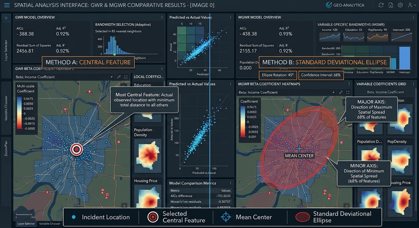
Two useful methods are Central Feature and Directional Distribution (Standard Deviational Ellipse). They examine the same dataset from different perspectives.

Central Feature identifies the actual observed feature that is most centrally located relative to the other features.
Directional Distribution creates an ellipse that summarizes the spatial distribution’s centre, spread, and orientation.

A related method, Mean Center, calculates the average geographic position of the input features. Comparing these outputs helps distinguish the average location from an actual observed location and from the overall direction of spatial dispersion.

These methods are available in ArcGIS Pro’s Measuring Geographic Distributions toolset, and comparable workflows are possible in QGIS using its native processing algorithms and plugins.

Common applications include:

Emergency planning: Summarizing incident locations and identifying central areas for further facility planning.
Environmental research: Examining the spatial distribution of wildlife sightings or pollution observations.
Urban analysis: Investigating the distribution of new developments or business locations.
Public health: Summarizing recorded disease cases geographically.
Retail planning: Comparing the distribution of stores and customer locations.

The key is to choose a tool based on the question you want to answer. An ellipse describes directional dispersion, while a central-feature analysis identifies an actual member of the dataset that minimizes accumulated distance. Understanding **Directional Distribution vs Central Feature GIS** methods helps researchers choose the right tool for spatial summaries.

2. Central Feature and Mean Center: Understanding Geographic Centrality

2.1 What is the Central Feature tool?

The Central Feature tool identifies the input feature with the smallest accumulated distance to all other features in the dataset, using the selected distance method. Reviewing Directional Distribution vs Central Feature GIS principles ensures you pick the correct summary method.

In simple terms, imagine calculating the distance from every incident location to every other incident location. For each feature, add up its distances to the remaining features. The feature with the smallest total is the Central Feature.

This produces an actual feature from the input dataset rather than an artificially calculated location.

For example, if a dataset contains 500 emergency incident points, Central Feature identifies the incident location that is most centrally positioned relative to the others under the selected distance method.

According to Esri’s Central Feature tool documentation, the output can contain more than one feature if several features share the minimum accumulated distance. When evaluating **Directional Distribution vs Central Feature GIS** outputs, comparing mean centers provides extra context.

2.2 How does Central Feature calculate the result?

The tool calculates distances between features and sums those distances for each candidate feature.

Two common distance methods are available in ArcGIS Pro:

Euclidean distance: Straight-line distance between locations.
Manhattan distance: Distance measured along perpendicular axes, similar to movement through a regular street grid.

For point features, the coordinates are used directly. For lines and polygons, the tool uses feature centroids in its distance calculations. If features have multiple parts, their centroids are calculated using the relevant geometry weighting.

A numeric weight field can also influence the analysis when meaningful weights are available. A case field can be used to identify a Central Feature for each group, such as each year or incident category.

When should you use Central Feature?

When you need an actual observed location rather than an estimated centre.
When selecting a representative incident, store, wildlife sighting, or other feature.
When comparing central observed features between groups.
When a straightforward distance-based summary is useful.

However, Central Feature does not automatically identify the best site for a new emergency response hub. Its distances are based on the selected mathematical distance method, not necessarily on road-network travel times, traffic, operational capacity, or access restrictions.

For a real facility-location decision, Central Feature is best treated as an initial spatial summary rather than a complete optimization method.

2.3 What is Mean Center?

The Mean Center calculates the average X and Y coordinates of the input features.

It produces a calculated location that summarizes the centre of the distribution. Unlike Central Feature, the result does not have to coincide with an existing feature.

For example, if several emergency incidents occur in different neighbourhoods, the mean center identifies their average geographic location.

Conceptually, the mean center is calculated by averaging all X-coordinates and all Y-coordinates separately.

You do not need to calculate the formula manually when using GIS software. The tool processes the input coordinates and creates the resulting point.

When should you use Mean Center?

When summarizing the average geographic location of a dataset.
When comparing the centre of incident distributions across years.
When investigating the shift in average wildlife observations between seasons.
When comparing distributions using weighted coordinates, if a meaningful numerical weight is available.

2.4 Central Feature vs. Mean Center

The difference is easier to understand with an example.

Suppose you have five store locations distributed across a city. Their average coordinate falls at a location between several stores.

Mean Center produces that calculated average point. Central Feature selects an actual store whose total distance to the other stores is the smallest.

The two points may be close together, but they answer different questions.

Feature	Central Feature	Mean Center
Output type	Existing input feature	Newly calculated point
Computation	Minimizes accumulated distances across observed features	Averages the coordinates of the features
Is the output an actual observation?	Yes	Not necessarily
Sensitivity to outliers	Depends on the distance pattern and feature weighting	Can be pulled toward distant observations
Typical application	Identifying an actual central store or incident	Summarizing the average location of a distribution
Main limitation	May be unsuitable as a real facility location	May fall in an inaccessible or unoccupied place

A related measure is the Median Center, which identifies a location minimizing the total distance to all features under its method. It is another calculated centre and can be useful when extreme observations may influence the mean center. ArcGIS Pro provides separate tools for these statistics; see the Measuring Geographic Distributions toolset.

3. Directional Distribution: Measuring Spatial Orientation

3.1 What is a Standard Deviational Ellipse?

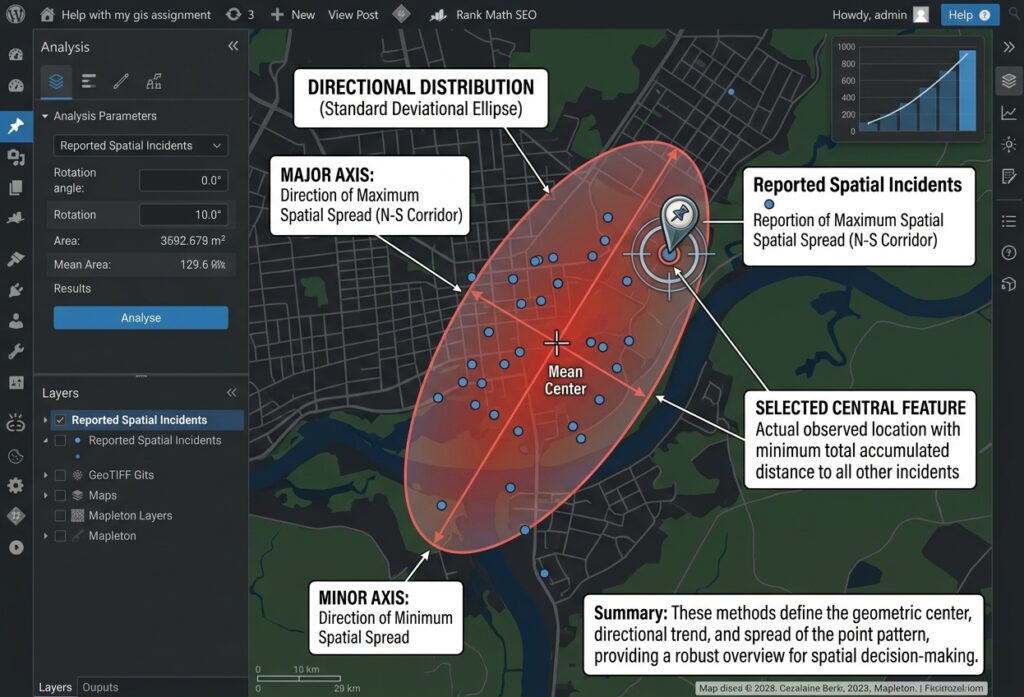
Directional Distribution, also called the Standard Deviational Ellipse (SDE), summarizes three properties of a geographic distribution:

Central tendency: The mean center of the observations.
Dispersion: How widely the observations are spread.
Directional orientation: The direction in which the distribution is most elongated.

The resulting ellipse provides a compact representation of the overall point pattern.

Imagine two groups of wildlife observations. The first group is spread similarly in all directions around its mean center. Its ellipse appears relatively circular. The second group follows a long valley, so its ellipse is elongated along the valley’s general direction.

This difference helps analysts describe spatial patterns in a way that is difficult to summarize from the point map alone. A comprehensive comparison within a Directional Distribution vs Central Feature GIS framework highlights both average coordinates and directional spread.

Esri explains the calculation and interpretation in its Directional Distribution documentation.

3.2 Understanding the ellipse axes

A standard deviational ellipse has two principal axes.

Major axis: The longer axis represents the direction of greatest spatial spread.

Minor axis: The shorter axis represents the direction of least spatial spread.

If the two axes are similar in length, the distribution is relatively circular. If the major axis is much longer than the minor axis, the data exhibit a stronger directional pattern.

The orientation angle describes the rotation of the ellipse’s major axis. In ArcGIS Pro, the Rotation field records the angle measured clockwise from noon, or north.

When comparing results from different GIS packages, verify their angle conventions because the direction of rotation and reference axis may differ.

3.3 How are the axes calculated?

The Directional Distribution algorithm calculates the variation in the X- and Y-coordinates around the mean center and the covariance between the two coordinates.

These quantities describe whether observations are spread independently in the coordinate directions or tend to align along a rotated direction.

The algorithm then determines the principal directions and corresponding standard-distance measures. These define the ellipse’s major and minor axes.

You do not need to calculate these values manually in a typical GIS workflow. The important task is to understand what the output represents and how to interpret it.

3.4 What do 1, 2, and 3 standard deviations mean?

ArcGIS Pro lets you choose an ellipse based on one, two, or three standard deviations.

Setting	General interpretation
1 standard deviation	Summarizes the central spatial spread
2 standard deviations	Shows a broader distribution
3 standard deviations	Shows a still broader extent, including more peripheral observations

For a spatial distribution that approximately follows the relevant bivariate normal model, ArcGIS Pro scales the ellipse to represent approximately 68%, 95%, and 99% of features for the one-, two-, and three-standard-deviation options, respectively.

These proportions are conditional on the distribution and implementation. They should not be interpreted as guaranteed coverage percentages for every geographic point pattern.

Important: The ellipse is a descriptive summary, not a boundary proving that all observations should fall inside it. Outliers may lie outside the ellipse, and an elongated ellipse does not prove movement in a particular direction.

3.5 Weighted Directional Distribution

If the observations have meaningful differences in importance, a numeric weight field can influence the ellipse calculation.

For example, an environmental study might assign weights based on a defensible measure of observation importance, while an incident study could investigate severity-weighted patterns.

Use weights only when they are justified by the research question. Weighting incidents by severity, for example, creates an ellipse that emphasizes more severe events rather than simply describing the distribution of all events equally.

4. Comparison Matrix: Central Feature vs. Directional Distribution

Feature	Central Feature	Mean Center	Directional Distribution
Output type	Actual input feature	Calculated point	Elliptical polygon
Primary purpose	Identify the most centrally located observation	Find the average geographic location	Measure centre, spread, and orientation
Computation	Minimum accumulated distance	Average X and Y coordinates	Coordinate dispersion and covariance
Main output properties	Selected feature and its attributes	Mean coordinates	Mean center, major/minor axes, orientation
Directional trend	Not directly measured	Not directly measured	Explicitly measured
Typical dataset	Store locations or incident points	Wildlife sightings or customer points	Storm observations, incident points, or urban features
Useful comparison	Compare central observed features by group	Compare average location across groups	Compare orientation and spread across groups

These methods complement one another. A useful analysis often calculates a mean center, identifies a Central Feature, and creates a Directional Distribution ellipse for the same dataset.

Together, the outputs describe where the distribution is centered, which observed feature is most central, and how the data are spread geographically.

5. Student Lab Project: Identifying a Candidate Emergency Response Hub

Suppose a city planning team has collected the locations of emergency incidents over the previous year. The objective is to summarize where incidents occur most centrally and whether their distribution follows a clear geographic orientation.

A suitable student workflow uses all three methods before considering where a new response hub might be located.

Step 1: Prepare the incident data

Collect a point dataset containing the recorded incident locations and, where relevant, attributes such as date, incident category, and severity.

Before analysis:

Verify the coordinate reference system.
Remove or correct duplicate and invalid records.
Confirm that incidents fall within the intended study area.
Decide whether every incident should have equal weight or whether a justified weighting scheme is needed.
If comparing years, confirm that the data-collection methods are sufficiently consistent.

Distance-based analysis should use an appropriate projected coordinate system for the study area. Working directly in longitude and latitude can lead to misleading distance measurements because those coordinates use angular units.

Step 2: Calculate the Mean Center

In ArcGIS Pro:

Open Analysis → Tools.
Search for Mean Center.
Select the incident point layer.
Specify the output feature class.
Add a year or incident-category case field if separate centers are needed.
Run the tool.

In QGIS:

Open the Processing Toolbox.
Search for Mean coordinate(s).
Select the incident layer and any justified weight field.
Choose a grouping field if required.
Save the output point layer.

The output indicates the average geographic location of the observed incidents.

Step 3: Identify the Central Feature

In ArcGIS Pro:

Open Analysis → Tools.
Search for Central Feature.
Select the incident point layer.
Choose Euclidean distance or Manhattan distance as appropriate.
Configure a weight field or case field if justified.
Run the tool.

In QGIS, the Spatial Analyzer plugin includes central-tendency methods such as Central Feature, Mean Center, and Median Center. Confirm the method, parameters, and compatibility with your QGIS version before using the result in a formal analysis.

The selected feature is the most centrally located observed incident under the chosen distance model. It is not necessarily the ideal location for a new response hub.

Step 4: Generate the Directional Distribution ellipse

In ArcGIS Pro:

Open Analysis → Tools.
Search for Directional Distribution (Standard Deviational Ellipse).
Select the incident layer.
Choose the ellipse size, such as one or two standard deviations.
Specify an output feature class.
Add a year field as the case field if you want separate ellipses by year.
Run the tool.

In QGIS:

Install a compatible Standard Deviational Ellipse tool, such as the Standard Deviational Ellipse plugin, or use the spatial dispersion functions provided by Spatial Analyzer.
Choose the input point layer and any appropriate grouping field.
Select the calculation method and ellipse size if available.
Run the analysis and inspect the ellipse attributes.

The ellipse reveals whether the incident pattern is compact or elongated and provides an orientation angle for the major axis.

Step 5: Interpret the results together

Imagine the results show:

The mean center is near the middle of the city.
The Central Feature is an incident location close to that center.
The ellipse is elongated along the city’s main transport corridor.

This suggests that incidents are distributed along a directional pattern rather than evenly around the centre.

The finding could help the planning team prioritize areas for additional investigation. However, it does not establish the optimal operating location for a response hub. Ultimately, comparing outcomes via **Directional Distribution vs Central Feature GIS** clarifies point dispersion patterns. Ultimately, contrasting outcomes using a Directional Distribution vs Central Feature GIS approach confirms your spatial orientation trends.

Step 6: Evaluate candidate response locations

To select a real emergency response hub, continue with a separate facility-location analysis.

Identify feasible candidate sites.
Consider road-network travel times instead of relying solely on straight-line distances.
Check land availability, access constraints, and operational requirements.
Evaluate response coverage and demand using a suitable network-analysis or location-allocation method.
Compare candidate sites against the operational objectives.

A Central Feature may serve as a useful point of reference, while the mean center and ellipse provide information about the incident distribution. The actual hub location should be determined from operational requirements and a suitable optimization method.

This distinction matters because the geographic centre of incidents is not automatically the location that minimizes emergency response times.

6. Common Mistakes to Avoid

Before writing your project report, check that you have avoided the following errors:

Treating the Central Feature as an optimal facility location. It minimizes accumulated distances to observed features under the selected distance method, not necessarily travel time on roads.
Confusing the Mean Center with the Central Feature. One is a calculated average coordinate; the other is an actual input feature.
Interpreting an ellipse as a movement trajectory. The ellipse describes dispersion and orientation, not the chronological path of individual events.
Ignoring the coordinate reference system. Distance and dispersion calculations should use suitable spatial units.
Comparing incompatible ellipse calculations. Use consistent methods, standard-deviation settings, weighting logic, and angle conventions when comparing years.
Overinterpreting outliers. Verify unusual locations before assuming they reflect a meaningful geographic process.

For an academic submission, document the input dataset, selected distance method, weights, grouping field, ellipse settings, projection, software tool, and the limitations of the analysis.

7. Conclusion

Central Feature and Directional Distribution are complementary tools for measuring geographic point patterns.

Central Feature identifies the actual observation with the smallest accumulated distance to the remaining features. Mean Center summarizes the average geographic location. Directional Distribution describes the location, spread, and orientation of the overall pattern using an ellipse.

For university GIS assignments, use Central Feature when an actual observed location is important, Mean Center when you need an average geographic reference point, and Directional Distribution when you want to summarize spatial dispersion and directional orientation.

The strongest analyses use the methods together, explain the distance and weighting assumptions, and interpret the results in the context of the research question.

The key lesson is that these tools describe the geometry of a spatial distribution. Additional analysis is needed to determine what causes that distribution or which real-world decision should follow from it.