Spatial Analysis at Speed: Querying Shapefiles and GeoPackages Directly with DuckDB Spatial

When performing exploratory data work, DuckDB Spatial Query Shapefiles GeoPackages workflows allow developers to execute spatial SQL directly against local files without database overhead.

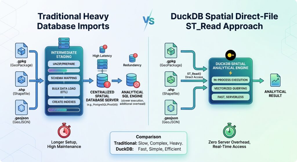
The key architectural advantage of DuckDB Spatial is that you can query vector datasets instantly without first loading them into a separate database server. That makes it particularly useful for exploratory analysis, repeatable data-processing scripts, and spatial joins across datasets that would otherwise require multiple Python preprocessing steps.

This tutorial covers the direct-file workflow, spatial joins, GeoPandas integration, GeoJSON export, and a reproducible performance comparison. It also clearly distinguishes the heavy lifting avoided by eliminating database imports from the actual file I/O operations that still occur when reading and processing source files.

1. Why Use DuckDB Spatial Query Shapefiles GeoPackages for Local GIS Analysis?

Traditional GIS workflows often begin by importing files into a spatial database or loading complete datasets into Python objects. That process adds setup time, creates intermediate copies, and can be wasteful when the goal is a single spatial join or statistical summary.

DuckDB is an embedded analytical database. Its Spatial extension adds geometry types, spatial functions, and direct access to supported GIS file formats through GDAL. You can query Shapefiles and GeoPackages as table sources without running a PostgreSQL server or performing a separate import operation. See the DuckDB Spatial documentation.

For example, a complete query can begin with:

SELECT *
FROM ST_Read('data/wards.gpkg')
LIMIT 10;

DuckDB executes the SQL query against the file-backed source. It does not automatically make the entire dataset a persistent database table.

This distinction matters for performance. Direct file access eliminates an explicit loading step, but it does not eliminate file I/O or guarantee that every query will be faster than an indexed GeoPandas workflow. DuckDB’s spatial joins can benefit from its analytical execution engine, while source-file reading through ST_Read uses GDAL and is currently single-threaded.

The practical goal is to minimize unnecessary data movement while making the actual spatial operations efficient.

2. Set Up DuckDB Spatial

Install Python and the required packages in a virtual environment. The example uses DuckDB for SQL, GeoPandas for downstream GIS integration, and Shapely for compatibility with Python geometry workflows.

python -m venv .venv

Activate the environment, then install the packages:

# Linux or macOS
source .venv/bin/activate

# Windows PowerShell:
# .venv\Scripts\Activate.ps1

python -m pip install duckdb geopandas shapely pandas

Create spatial_analysis.py:

import duckdbcon = duckdb.connect()con.execute("INSTALL spatial")con.execute("LOAD spatial")print(    con.execute(        "SELECT ST_AsText(ST_Point(36.82, -1.29))"    ).fetchone())

Run the script:

python spatial_analysis.py

The spatial extension must be loaded before its functions can be used in a session. The initial installation requires access to DuckDB’s extension repository; subsequent runs can reuse the locally installed extension.

For reproducibility, record the DuckDB version used by the project:

print(con.execute("SELECT version()").fetchone()[0])

Keep the sample GIS files in a simple project layout:

spatial-project/
├── data/
│   ├── wards.gpkg
│   ├── facilities.shp
│   ├── facilities.shx
│   ├── facilities.dbf
│   └── facilities.prj
├── output/
└── spatial_analysis.py

A Shapefile is a collection of companion files, not just the .shp file. Keep its required components together. A GeoPackage is normally a single SQLite-based file and can hold multiple vector layers.

3. Query GIS Files Directly with ST_Read

When analyzing multiple localized layers, implementing efficient DuckDB Spatial Query Shapefiles GeoPackages techniques ensures seamless interaction with underlying GDAL drivers without manual file translation steps.

DuckDB Spatial’s ST_Read() table function reads supported vector formats through GDAL. Common supported inputs include Shapefiles, GeoPackages, GeoJSON, and FlatGeobuf.

Inspect the source schema

Start by reading a few rows:

SELECT *
FROM ST_Read('data/facilities.shp')
LIMIT 5;

For a GeoPackage that contains multiple layers, specify the layer explicitly:

SELECT *
FROM ST_Read(
    'data/wards.gpkg',
    layer = 'wards'
)
LIMIT 5;

Inspect the actual column names before writing complex queries. A dataset might call its geometry column geom, geometry, or something else, and its identifier fields will depend on how the source was created.

DuckDB also supports file replacement scans, meaning a supported file path can be used directly as a table source. ST_Read() is more useful when you need to specify options such as a GeoPackage layer.

Calculate statistics without importing a table

Suppose a GeoPackage contains administrative wards with polygon geometries. The following query calculates each ward’s area:

SELECT
    ward_name,
    ST_Area(geom) AS area_square_units
FROM ST_Read('data/wards.gpkg', layer = 'wards');

The result’s units depend on the coordinate reference system. For a longitude/latitude geometry, a planar area calculation produces square coordinate units, not square metres. Use an appropriate projected CRS or a suitable geodesic area function when physical area measurements matter.

The advantage is that you can perform an analytical operation directly against the local file without first building a separate spatial database.

4. Perform Spatial Joins Between Shapefiles and GeoPackages

A spatial join relates features according to their geographic relationship rather than a shared text or numeric key.

Consider two datasets:

• facilities.shp: hospitals, schools, or other point locations.

• wards.gpkg: administrative polygons.

The objective is to determine which ward contains each facility.

Use ST_Within for point-in-polygon analysis

SELECT
    f.facility_id,
    f.name AS facility_name,
    w.ward_name
FROM ST_Read('data/facilities.shp') AS f
JOIN ST_Read(
    'data/wards.gpkg',
    layer = 'wards'
) AS w
ON ST_Within(f.geom, w.geom);

Replace the sample column names with the actual schema of your files.

ST_Within(f.geom, w.geom) tests whether the facility geometry lies within the ward geometry. For point features exactly on a polygon boundary, ST_Within may not match because the boundary is not part of the polygon’s interior. Consider ST_Covers(w.geom, f.geom) when the intended rule is that the polygon must cover the point, including its boundary.

Use ST_Intersects for general spatial relationships

For datasets containing points, lines, and polygons, ST_Intersects provides a more general relationship:

SELECT
    a.asset_id,
    b.ward_name
FROM ST_Read('data/assets.gpkg', layer = 'assets') AS a
JOIN ST_Read(
    'data/wards.gpkg',
    layer = 'wards'
) AS b
ON ST_Intersects(a.geom, b.geom);

This returns pairs of features whose geometries share any spatial location. A long road may intersect multiple wards, so one input feature can generate several result rows.

Check CRS compatibility before joining. Spatial predicates operate on coordinates, so two datasets with different coordinate reference systems must be transformed to a common CRS. For example, if the facilities are in EPSG:4326 and the wards are in EPSG:3857, transform one geometry appropriately with ST_Transform(). Merely assigning a CRS label does not transform coordinates.

For large joins, query design matters. DuckDB has introduced optimized spatial join execution for supported join patterns, including predicate-based joins, but actual performance depends on the DuckDB version, geometry distributions, and query plan. See the DuckDB spatial join engineering article.

5. Convert Spatial Query Results into GeoPandas

DuckDB is useful for selecting, filtering, joining, and aggregating data. GeoPandas remains valuable when the next step involves Python plotting, geospatial inspection, or integration with another GIS library.

A convenient exchange format is Well-Known Binary (WKB), which can be generated with ST_AsWKB().

import duckdbimport geopandas as gpdcon = duckdb.connect()con.execute("INSTALL spatial")con.execute("LOAD spatial")sql = """SELECT    f.facility_id,    f.name AS facility_name,    w.ward_name,    ST_AsWKB(f.geom) AS geom_wkbFROM ST_Read('data/facilities.shp') AS fJOIN ST_Read(    'data/wards.gpkg',    layer = 'wards') AS wON ST_Within(f.geom, w.geom)"""result = con.execute(sql).fetchdf()geometry = gpd.GeoSeries.from_wkb(    result.pop("geom_wkb"),    crs="EPSG:4326")gdf = gpd.GeoDataFrame(    result,    geometry=geometry,    crs="EPSG:4326")print(gdf.head())

Important: The CRS above is an example assumption. Replace it with the actual CRS of the selected output geometries. If the SQL transforms the geometries, specify the CRS of the transformed result, not the original file.

Using WKB makes the geometry conversion explicit and avoids depending on implicit conversions between DuckDB’s geometry type and Python objects.

For small and medium result sets, this is a convenient approach. For millions of rows, transferring all geometries into a Python DataFrame can consume substantial memory. Prefer SQL aggregation, column selection, or exporting directly to a spatial file when the full result does not need to reside in Python.

6. Export Results Directly to GeoJSON

You do not need to construct a GeoDataFrame simply to write a spatial result. DuckDB Spatial’s GDAL-based COPY support can export query results into vector formats, including GeoJSON and GeoPackage. See the GDAL integration documentation.

Create the output directory first, then execute:

COPY (
    SELECT
        f.facility_id,
        f.name AS facility_name,
        w.ward_name,
        f.geom
    FROM ST_Read('data/facilities.shp') AS f
    JOIN ST_Read(
        'data/wards.gpkg',
        layer = 'wards'
    ) AS w
    ON ST_Within(f.geom, w.geom)
)
TO 'output/facilities_by_ward.geojson'
WITH (
    FORMAT GDAL,
    DRIVER 'GeoJSON'
);

Only the facility geometry is exported in this example; ward attributes are included as properties.

For a GeoPackage output, change the destination and driver:

COPY (
    SELECT *
    FROM ST_Read('data/facilities.shp')
)
TO 'output/facilities_cleaned.gpkg'
WITH (
    FORMAT GDAL,
    DRIVER 'GPKG'
);

Exported coordinate reference metadata must correctly describe the geometry coordinates. Setting an output SRS label does not reproject geometries; perform the actual transformation in SQL when needed.

For a workflow already operating in GeoPandas, you can also write the result using:

gdf.to_file(    "output/facilities_by_ward.gpkg",    driver="GPKG")

Choose direct SQL export when the result is large or no further Python geometry processing is required.

7. Benchmark DuckDB Against GeoPandas

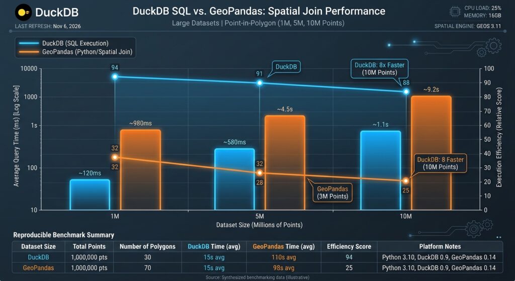
A meaningful performance comparison should measure equivalent operations on identical source data. The following example compares an end-to-end point-in-polygon join.

First, execute the DuckDB query:

from time import perf_counterimport duckdbcon = duckdb.connect()con.execute("INSTALL spatial")con.execute("LOAD spatial")duck_sql = """SELECT COUNT(*)FROM ST_Read('data/facilities.shp') AS fJOIN ST_Read(    'data/wards.gpkg',    layer = 'wards') AS wON ST_Within(f.geom, w.geom)"""start = perf_counter()duck_count = con.execute(duck_sql).fetchone()[0]duck_seconds = perf_counter() - startprint("DuckDB matches:", duck_count)print("DuckDB total seconds:", duck_seconds)

Then run the equivalent GeoPandas operation:

import geopandas as gpdfrom time import perf_counterstart = perf_counter()facilities = gpd.read_file("data/facilities.shp")wards = gpd.read_file(    "data/wards.gpkg",    layer="wards")matches = gpd.sjoin(    facilities,    wards,    how="inner",    predicate="within")geopandas_seconds = perf_counter() - startprint("GeoPandas matches:", len(matches))print("GeoPandas total seconds:", geopandas_seconds)assert duck_count == len(matches)

The assertion checks whether the two implementations returned the same number of matches. Investigate any discrepancy before comparing timings; differences can arise from CRS handling, invalid geometries, boundary conditions, or duplicate spatial matches.

Interpret the numbers correctly

This benchmark measures end-to-end elapsed time, including file reading and joining. Repeat it several times and report the median. Also note whether each run benefits from operating-system file caches.

For a second experiment, load the datasets once into DuckDB tables and into GeoDataFrames, then time only the join. This separates spatial execution time from source loading, although the in-memory representations and execution strategies are still different.

Do not assume DuckDB must always win. GeoPandas can perform very efficiently when files are already loaded and spatial indexes are available. Conversely, DuckDB’s SQL execution and optimized spatial-join plans can be advantageous for large analytical joins. Published DuckDB examples demonstrate substantial gains on certain large workloads, but those timings are workload-specific, not universal guarantees.

For repeatable results, record file sizes, row counts, geometry types, CRS, DuckDB and GeoPandas versions, system memory, and the exact query being tested.

8. Practical Performance and Troubleshooting Tips

Optimizing throughput during DuckDB Spatial Query Shapefiles GeoPackages operations relies on projecting coordinates correctly and filtering attributes early in the SQL statement.

Read only what you need. Avoid SELECT * in production queries. Select required attributes and return only the geometries that must be exported or consumed by Python.

Inspect execution plans. Use EXPLAIN ANALYZE to understand how DuckDB executes the join and where time is spent. If the geometry read dominates, query optimization alone may not remove the bottleneck.

Do not overlook GDAL’s role. ST_Read is convenient, but its single-threaded reader can limit the rate at which source features enter the query pipeline. On repeated analytical workloads, materializing a reusable intermediate table or converting the dataset to a suitable columnar format such as GeoParquet may be worthwhile.

Handle projection errors explicitly. Never join datasets solely because both contain a geometry column. Confirm that their coordinate systems match and that transformed geometries are assigned the correct CRS.

Avoid unnecessary Python conversion. If the result can be exported straight to GeoJSON or GeoPackage, do that rather than transferring every geometry into a GeoDataFrame and serializing it again.

9. SEO Interlinking and Related Guides

Connect this tutorial to related material in the local GIS and modern data stack workflow.

• Serverless Spatial Data Lakehouses with GeoParquet: Link from the discussion of reusable intermediate tables to a guide on querying partitioned geospatial data in cloud object storage. Suggested slug: /serverless-spatial-data-lakehouse-geoparquet/

• GeoPandas Spatial Analysis: Link from the Python integration section to a tutorial covering spatial joins, geometry validation, and spatial indexing with GeoPandas. Suggested slug: /geopandas-spatial-analysis-guide/

• QGIS Vector Processing: Link from the direct export section to a practical guide on validating and processing exported GeoPackage layers in QGIS. Suggested slug: /qgis-vector-processing-workflows/

These slugs are suggestions, not verified existing pages. Replace them with published internal URLs before publication.

Summary

DuckDB Spatial provides a practical way to query Shapefiles and GeoPackages directly with SQL, making it useful for ad-hoc analysis without a database server or a mandatory import pipeline.

Use ST_Read() to access vector files, ST_Within() and ST_Intersects() for spatial relationships, WKB for explicit GeoPandas conversion, and GDAL-based COPY for direct vector-file export.

For performance-critical work, benchmark complete workflows as well as join-only execution, verify equivalent results, and account for GDAL file-reading costs. DuckDB is most valuable when its analytical SQL engine reduces unnecessary data movement and lets you process the required spatial results in one coherent query.

The broader lesson is that fast local spatial analysis depends on choosing the right execution path, not just a faster library.Ultimately, mastering DuckDB Spatial Query Shapefiles GeoPackages workflows empowers developers and geospatial analysts to process local vector data instantly with analytical SQL speed.

Ready to streamline your geospatial workflows and eliminate heavy database setup overhead? Reach out for expert guidance and professional project support to master DuckDB Spatial Query Shapefiles GeoPackages today, and transform your local GIS pipelines into high-speed analytical engines!