
How to Calculate Spatial Distance Matrices with Python SciPy and Shapely
How to Calculate Spatial Distance Matrices with Python SciPy and Shapely is essential for mastering spatial distance calculations in GIS workflows. Whether you are determining which hospital is closest to a patient, matching warehouses to customers, or analyzing the nearest neighboring features, calculating distances between many points is a common requirement.
Python provides an efficient combination of GeoPandas, Shapely, and SciPy for these workflows.
This tutorial demonstrates how to build a Spatial Distance Matrix Python GeoPandas scipy workflow, calculate pairwise distances between two point datasets, identify the nearest destination for every origin, and export the results for further GIS or statistical analysis.
1. Introduction: How to Calculate Spatial Distance Matrices with Python SciPy and Shapely
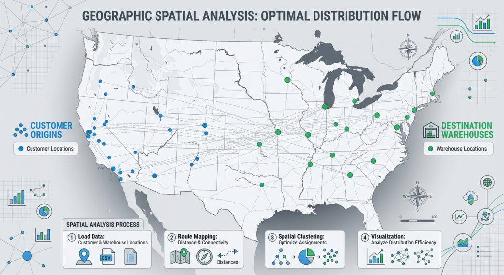
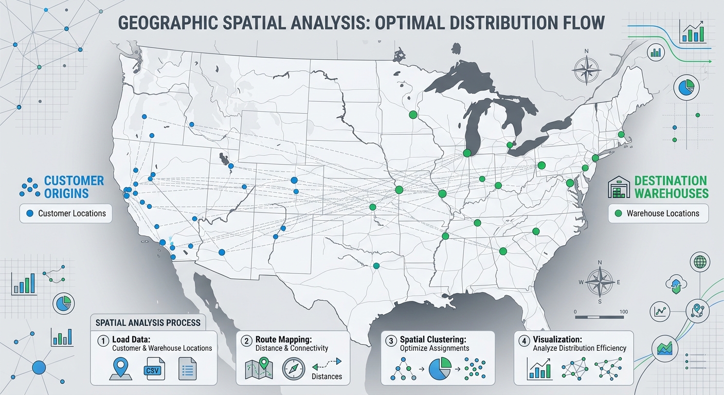
A spatial distance matrix is a table or numerical array containing the distances between two or more sets of geographic features.
Suppose you have:
- 4 demand points representing customers
- 3 destination points representing warehouses
The resulting matrix could look like this:
| Warehouse 1 | Warehouse 2 | Warehouse 3 | |
|---|---|---|---|
| Customer 1 | 2,150 m | 5,430 m | 3,210 m |
| Customer 2 | 1,870 m | 4,100 m | 2,950 m |
| Customer 3 | 6,210 m | 2,300 m | 1,540 m |
| Customer 4 | 3,450 m | 1,980 m | 4,220 m |
Each row represents an origin, while each column represents a destination.
Mathematically, if there are n origins and m destinations, the distance matrix has dimensions:
\[ n \times m \]
For example:
100 origins × 20 facilitiesproduces:
100 × 20or 2,000 individual distance calculations.
Why are distance matrices useful?
Distance matrices are important in:
- Facility location models
- Supply-chain logistics
- Emergency-service planning
- Transportation analysis
- Nearest-neighbor analysis
- Customer-to-store allocation
- Healthcare accessibility studies
- School location analysis
- Spatial clustering
- Network planning
A common question is:
“For every demand point, which facility is closest?”
A distance matrix gives you everything needed to answer that question.
2. Setup and Required Libraries
We will use three primary geospatial/scientific Python libraries:
import geopandas as gpd
from shapely.geometry import Point
from scipy.spatial.distance import cdist
Each library has a different role.
GeoPandas
GeoPandas handles spatial datasets and coordinate reference systems.
import geopandas as gpdWe will use it to:
- Read GIS files
- Manage GeoDataFrames
- Reproject coordinates
- Work with geometry columns
Shapely
Shapely provides geometric objects such as points, lines, and polygons.
from shapely.geometry import PointIn this tutorial, the geometries are already stored in our GeoDataFrames, so Shapely mainly provides the underlying geometry functionality.
SciPy
SciPy provides optimized scientific-computing algorithms.
from scipy.spatial.distance import cdistcdist() is particularly useful because it calculates the distances between every point in one dataset and every point in another dataset.
Install the libraries if necessary:
pip install geopandas shapely scipy3. Example Dataset
Imagine a logistics company with two spatial datasets:
Origins
These represent customer demand locations.
origins.gpkgExample attributes:
| Origin_ID | Demand | geometry |
|---|---|---|
| O001 | 150 | Point |
| O002 | 320 | Point |
| O003 | 210 | Point |
| O004 | 450 | Point |
Destinations
These represent warehouses.
facilities.gpkgExample attributes:
| Facility_ID | Capacity | geometry |
|---|---|---|
| F001 | 5000 | Point |
| F002 | 3000 | Point |
| F003 | 7000 | Point |
Our goal is to calculate the distance from every origin to every facility.
4. Step 1 — Load the Point Datasets
Start by importing GeoPandas:
import geopandas as gpdRead the two datasets:
origins = gpd.read_file("origins.gpkg")
facilities = gpd.read_file("facilities.gpkg")
Inspect them:
print(origins.head())
print(facilities.head())
You can also check their coordinate reference systems:
print("Origins CRS:", origins.crs)
print("Facilities CRS:", facilities.crs)
You might find:
Origins CRS: EPSG:4326
Facilities CRS: EPSG:4326
This means the coordinates are stored as longitude and latitude.
That creates an important problem.
5. Step 2 — Project the Data to a CRS Using Meters
Do not calculate Euclidean distance directly from latitude/longitude.
Coordinates in:
EPSG:4326are expressed in degrees.
For example:
Longitude = 36.8172
Latitude = -1.2864
A difference of 0.01 degrees does not represent a fixed distance in meters across the Earth’s surface.
For Euclidean distance calculations, we therefore want a projected CRS whose units are meters.
For a Kenyan study area, for example, you might use an appropriate UTM CRS for your area of interest.
Suppose our data is in a suitable projected CRS:
EPSG:32737You could reproject both datasets:
origins_projected = origins.to_crs("EPSG:32737")
facilities_projected = facilities.to_crs("EPSG:32737")
Now check the CRS:
print(origins_projected.crs)The coordinates are now represented in meters.
Important: The projected CRS should be appropriate for your study area. Do not blindly use one EPSG code for every project.
6. Why the CRS Matters
Suppose two points have coordinates:
Point A: (500000, 9850000)
Point B: (501000, 9851000)
Because the coordinates are in meters, we can calculate the Euclidean distance:
\[ d = \sqrt{(x_2-x_1)^2 + (y_2-y_1)^2} \]
Therefore:
\[ d = \sqrt{1000^2 + 1000^2} \]
which gives approximately:
1,414.21 metersThis is exactly the type of calculation that scipy.spatial.distance.cdist() performs efficiently.
7. Step 3 — Extract X and Y Coordinates
SciPy does not directly calculate distances from GeoPandas geometry objects.
We first extract the coordinates into numerical arrays.
For the origins:
origin_coords = [
    [point.x, point.y]
    for point in origins_projected.geometry
]
For the facilities:
facility_coords = [
    [point.x, point.y]
    for point in facilities_projected.geometry
]
You can inspect the result:
print(origin_coords[:3])
print(facility_coords[:3])
You should see something similar to:
[[500123.4, 9850123.7],
 [501230.8, 9851450.2],
 [498765.1, 9849320.6]]
These are ordinary numerical coordinate pairs.
8. Step 4 — Convert Coordinates into Arrays
For larger datasets, NumPy arrays are preferable.
Import NumPy:
import numpy as npThen:
origin_coords = np.array([
    [point.x, point.y]
    for point in origins_projected.geometry
])

facility_coords = np.array([
    [point.x, point.y]
    for point in facilities_projected.geometry
])
Now inspect their dimensions:
print(origin_coords.shape)
print(facility_coords.shape)
Suppose we have:
100 origins
20 facilities
The result would be:
(100, 2)
(20, 2)
The 2 represents:
X coordinate
Y coordinate
9. Step 5 — Calculate the Spatial Distance Matrix

Now we can use SciPy’s cdist().
from scipy.spatial.distance import cdistCalculate the distances:
distance_matrix = cdist(
    origin_coords,
    facility_coords,
    metric="euclidean"
)
This single operation calculates every origin-to-facility distance.
If there are:
100 origins
20 facilities
the resulting matrix has:
100 rows × 20 columnsCheck its shape:
print(distance_matrix.shape)Output:
(100, 20)10. Understanding cdist()
The basic syntax is:
cdist(A, B, metric="euclidean")where:
A= coordinates of the first datasetB= coordinates of the second datasetmetric= distance calculation method
In our case:
distance_matrix = cdist(
    origin_coords,
    facility_coords,
    metric="euclidean"
)
Conceptually, SciPy calculates:
Origin 1 → Facility 1
Origin 1 → Facility 2
Origin 1 → Facility 3

Origin 2 → Facility 1
Origin 2 → Facility 2
Origin 2 → Facility 3

...
until every combination has been calculated.
11. Inspect the Distance Matrix
You can print the matrix:
print(distance_matrix)For example:
[[2150.4 5430.7 3210.2]
 [1870.5 4100.1 2950.6]
 [6210.8 2300.4 1540.7]
 [3450.2 1980.6 4220.3]]
The first row corresponds to the first origin.
The columns correspond to the facilities.
Therefore:
distance_matrix[0, 0]means:
Origin 1 → Facility 1while:
distance_matrix[0, 1]means:
Origin 1 → Facility 212. Step 6 — Find the Nearest Destination
A common requirement is not the entire matrix but simply the closest destination for every origin.
NumPy’s argmin() is useful here.
nearest_indices = np.argmin(
    distance_matrix,
    axis=1
)
Why axis=1?
Each row represents one origin.
We want to find the minimum value within each row.
For example:
Origin 1:
[2150, 5430, 3210]
The smallest value is:
2150and its column index is:
0Therefore, Facility 1 is the nearest facility.
13. Extract the Minimum Distance
We can obtain the actual minimum distance using:
minimum_distances = np.min(
    distance_matrix,
    axis=1
)
Now we have two arrays:
nearest_indices
minimum_distances
For example:
nearest_indices:
[0, 0, 2, 1]

minimum_distances:
[2150.4, 1870.5, 1540.7, 1980.6]
This tells us which facility is nearest and how far away it is.
14. Step 7 — Match the Index to the Facility ID
The argmin() result gives us a position, not necessarily the actual facility ID.
Suppose:
facilities_projected["Facility_ID"]contains:
F001
F002
F003
We can use the indices:
nearest_facilities = facilities_projected.iloc[
    nearest_indices
]["Facility_ID"].values
Now:
nearest_indicesmight be:
[0, 0, 2, 1]while:
nearest_facilitiesbecomes:
["F001", "F001", "F003", "F002"]15. Step 8 — Create a Results Table
We can now construct a pandas DataFrame.
import pandas as pd

results = pd.DataFrame({
    "Origin_ID": origins_projected["Origin_ID"].values,
    "Nearest_Facility": nearest_facilities,
    "Distance_m": minimum_distances
})
Inspect the result:
print(results.head())You might get:
| Origin_ID | Nearest_Facility | Distance_m |
|---|---|---|
| O001 | F001 | 2150.4 |
| O002 | F001 | 1870.5 |
| O003 | F003 | 1540.7 |
| O004 | F002 | 1980.6 |
This table can now be used for statistical analysis, reporting, or GIS visualization.
16. Export the Nearest-Destination Results
Save the table as CSV:
results.to_csv(
    "nearest_facilities.csv",
    index=False
)
The resulting file might look like:
Origin_ID,Nearest_Facility,Distance_m
O001,F001,2150.4
O002,F001,1870.5
O003,F003,1540.7
O004,F002,1980.6
You can open this in Excel, QGIS, ArcGIS Pro, pandas, or another analytical system.
17. Export the Complete Distance Matrix
Sometimes you need every origin-to-destination distance, not just the nearest facility.
One convenient approach is to use the destination IDs as column names.
distance_df = pd.DataFrame(
    distance_matrix,
    index=origins_projected["Origin_ID"],
    columns=facilities_projected["Facility_ID"]
)
Inspect it:
print(distance_df.head())The result might look like:
| Origin_ID | F001 | F002 | F003 |
|---|---|---|---|
| O001 | 2150 | 5431 | 3210 |
| O002 | 1871 | 4100 | 2951 |
| O003 | 6211 | 2300 | 1541 |
| O004 | 3450 | 1981 | 4220 |
Export it:
distance_df.to_csv(
    "spatial_distance_matrix.csv"
)
You now have a complete Spatial Distance Matrix Python GeoPandas scipy output.
18. Complete Workflow Script
Here is the complete workflow assembled into one script:
import geopandas as gpd
import pandas as pd
import numpy as np
from scipy.spatial.distance import cdist


# --------------------------------------------------
# 1. Load datasets
# --------------------------------------------------

origins = gpd.read_file("origins.gpkg")
facilities = gpd.read_file("facilities.gpkg")


# --------------------------------------------------
# 2. Project both datasets to a CRS in meters
# --------------------------------------------------

target_crs = "EPSG:32737"

origins_projected = origins.to_crs(target_crs)
facilities_projected = facilities.to_crs(target_crs)


# --------------------------------------------------
# 3. Extract X/Y coordinates
# --------------------------------------------------

origin_coords = np.array([
    [point.x, point.y]
    for point in origins_projected.geometry
])

facility_coords = np.array([
    [point.x, point.y]
    for point in facilities_projected.geometry
])


# --------------------------------------------------
# 4. Calculate pairwise distances
# --------------------------------------------------

distance_matrix = cdist(
    origin_coords,
    facility_coords,
    metric="euclidean"
)


# --------------------------------------------------
# 5. Find nearest facility for each origin
# --------------------------------------------------

nearest_indices = np.argmin(
    distance_matrix,
    axis=1
)

minimum_distances = np.min(
    distance_matrix,
    axis=1
)


# --------------------------------------------------
# 6. Convert facility indices to IDs
# --------------------------------------------------

nearest_facilities = facilities_projected.iloc[
    nearest_indices
]["Facility_ID"].values


# --------------------------------------------------
# 7. Create nearest-facility results
# --------------------------------------------------

results = pd.DataFrame({
    "Origin_ID": origins_projected["Origin_ID"].values,
    "Nearest_Facility": nearest_facilities,
    "Distance_m": minimum_distances
})


# --------------------------------------------------
# 8. Save nearest-facility table
# --------------------------------------------------

results.to_csv(
    "nearest_facilities.csv",
    index=False
)


# --------------------------------------------------
# 9. Create complete distance matrix
# --------------------------------------------------

distance_df = pd.DataFrame(
    distance_matrix,
    index=origins_projected["Origin_ID"],
    columns=facilities_projected["Facility_ID"]
)


# --------------------------------------------------
# 10. Save complete matrix
# --------------------------------------------------

distance_df.to_csv(
    "spatial_distance_matrix.csv"
)


# --------------------------------------------------
# 11. Print summary
# --------------------------------------------------

print("Distance calculation completed.")
print(f"Origins: {len(origins_projected)}")
print(f"Facilities: {len(facilities_projected)}")
print(f"Matrix shape: {distance_matrix.shape}")
19. Performance Considerations
The main limitation of a full distance matrix is size.
If you have:
1,000 origins
500 facilities
you need:
\[ 1,000 \times 500 = 500,000 \]
distance calculations.
That is manageable.
But consider:
100,000 origins
50,000 facilities
The matrix would contain:
\[ 100,000 \times 50,000 = 5,000,000,000 \]
distance values.
That is 5 billion values, which can require enormous amounts of memory.
Therefore, you should not automatically create a full matrix for very large datasets.
20. Estimate Matrix Memory
A NumPy float64 value requires approximately 8 bytes.
You can estimate memory requirements:
n_origins = len(origins_projected)
n_facilities = len(facilities_projected)

memory_bytes = (
    n_origins *
    n_facilities *
    8
)

memory_gb = memory_bytes / (1024 ** 3)

print(
    f"Estimated matrix size: "
    f"{memory_gb:.2f} GB"
)
This is a useful check before running cdist() on a large dataset.
21. When You Only Need the Nearest Neighbor
If your actual question is:
“Which facility is closest to each origin?”
you may not need to generate every possible origin-to-facility distance.
GeoPandas provides spatial nearest-neighbor functionality that can be more appropriate for this type of problem.
For example:
nearest = gpd.sjoin_nearest(
    origins_projected,
    facilities_projected,
    how="left",
    distance_col="Distance_m"
)
This directly performs a nearest spatial join.
For very large datasets, this type of spatial-index-based approach can be substantially more appropriate than constructing a massive dense distance matrix.
22. Pairwise Distance Calculation vs Nearest Neighbor
These approaches answer slightly different questions.
| Task | Suitable approach |
|---|---|
| Every origin-to-every-facility distance | scipy.spatial.distance.cdist() |
| Find nearest facility | gpd.sjoin_nearest() |
| Calculate all distances for a small dataset | cdist() |
| Very large nearest-neighbor problem | Spatial index / nearest join |
| Statistical distance analysis | Distance matrix |
| Facility allocation modeling | Distance matrix or optimized nearest search |
The key is to choose the algorithm based on the analytical question rather than automatically generating the largest possible matrix.
23. Important Distance Limitation
The cdist() workflow calculates Euclidean distance between projected coordinates.
That means:
straight-line distanceIt does not calculate:
road distance
driving distance
travel time
walking distance
For example, two locations might be 2 km apart in Euclidean space but 5 km apart by road because of rivers, highways, restricted areas, or the street network.
Therefore:
Use
cdist()when straight-line distance is appropriate to your analysis.
For transportation and logistics applications where actual travel distance matters, a network analysis workflow is usually more appropriate.
24. Conclusion
A spatial distance matrix provides a structured way to quantify the relationship between locations.
Using GeoPandas, Shapely, NumPy, and SciPy, the basic workflow is:
Load spatial datasets
        ↓
Project to a suitable CRS
        ↓
Extract X/Y coordinates
        ↓
Create coordinate arrays
        ↓
Calculate pairwise distances
        ↓
Find minimum distances
        ↓
Match nearest destination IDs
        ↓
Export results
The core calculation is remarkably compact:
distance_matrix = cdist(
    origin_coords,
    facility_coords,
    metric="euclidean"
)
And finding the nearest destination for each origin requires only:
nearest_indices = np.argmin( distance_matrix, axis=1)minimum_distances = np.min( distance_matrix, axis=1)The most important considerations are CRS selection, coordinate order, matrix size, and choosing Euclidean distance versus network distance.
Once you understand this workflow, you can extend it to facility location models, supply-chain optimization, accessibility analysis, and nearest neighbor analysis in Python without manually calculating individual GIS distances.
Frequently Asked Questions
What tools are required for How to Calculate Spatial Distance Matrices with Python SciPy and Shapely?
To run this workflow, you need GeoPandas for reading and managing spatial files, Shapely for geometry handling, NumPy for array structuring, and SciPy’s `cdist` function for high-speed pairwise calculations.
Why is data projection important when learning How to Calculate Spatial Distance Matrices with Python SciPy and Shapely?
Unprojected latitude and longitude coordinates (like EPSG:4326) measure positions in degrees, which do not translate to uniform meter distances. Reprojecting your origins and facilities to a local metric CRS (such as UTM) ensures your Euclidean distance matrix is accurate.