
Mapping Groundwater Potential Zones Using Analytical Hierarchy Process (AHP) in GIS
GIS Research Guide · Hydrogeology · Multi-Criteria Decision Analysis · QGIS & ArcGIS Pro
Introduction
Groundwater is a critical source of freshwater for domestic consumption, agriculture, and industrial development. However, identifying productive groundwater zones is challenging because groundwater occurrence depends on several interacting factors, including geology, terrain, rainfall, surface drainage, and the presence of fractures in underlying rocks.
In many regions, groundwater exploration relies on geological surveys, geophysical investigations, borehole drilling, and hydrogeological field studies. These approaches provide important evidence but can be expensive and difficult to apply uniformly across large areas.
Groundwater Potential Mapping AHP GIS combines remote sensing, spatial analysis, and the Analytical Hierarchy Process (AHP) to identify areas with relatively favourable conditions for groundwater occurrence and development. AHP assigns relative importance to selected environmental factors, while GIS combines their spatial representations into a groundwater potential map. Research has demonstrated the usefulness of this approach in different hydrogeological environments, including semi-arid catchments.

The central idea is to transform different datasets into comparable suitability scores, assign scientifically justified weights to each factor, and combine the results to produce a spatial index of groundwater potential.
It is important to distinguish groundwater potential from groundwater recharge potential. Groundwater potential mapping typically estimates where groundwater is more likely to occur or where productive wells may be found. Recharge potential mapping focuses more specifically on areas where water can infiltrate and replenish aquifers. The two are related, but they are not identical.
Objectives of the analysis
This guide explains how to:
-
Select six important groundwater-related spatial factors.
-
Calculate criterion weights using Saaty’s AHP method.
-
Check the consistency of pairwise comparisons.
-
Prepare and reclassify thematic raster layers in QGIS or ArcGIS Pro.
-
Apply weighted overlay to generate a groundwater potential index.
-
Delineate low, moderate, and high potential zones.
-
Validate the resulting map using borehole yield data.
The example uses six criteria and a hypothetical study area. Its numerical weights are illustrative, not universal hydrogeological constants. Real projects should adapt their criteria, ratings, and weights to local geology, climate, aquifer conditions, and available evidence.
1. Selecting the key groundwater potential factors
Before performing the AHP calculations, define which environmental variables will influence the model. The six criteria below are widely used in groundwater potential studies, although their relative importance varies between study areas.

1. Lithology
Lithology describes the mineral composition and physical characteristics of rocks and geological materials. It influences groundwater storage, permeability, and transmission.
Mapping approach: Obtain a geological map, digitize relevant rock units if necessary, and assign suitability scores based on local evidence of porosity, permeability, weathering, and fracturing.
General guidance: Permeable sedimentary formations and productive weathered or fractured rocks may receive higher scores. Clay-rich or otherwise poorly permeable units may receive lower scores, depending on the local hydrogeology.

2. Land Use/Land Cover (LULC)
LULC influences infiltration, surface runoff, soil disturbance, and the likelihood of contamination.
Mapping approach: Classify satellite imagery or use an existing land-cover dataset.
General guidance: Vegetated and permeable surfaces may promote infiltration. Impervious urban areas may reduce recharge, while agricultural land can have variable infiltration and contamination risks. Assign scores according to the objective of the study and local conditions.

3. Drainage density
Drainage density is the total length of mapped stream channels per unit area. It provides information about runoff, terrain, and the surface expression of subsurface conditions.
Mapping approach: Derive a stream network from a DEM or use a reliable hydrographic dataset, then calculate drainage density using line-density or equivalent spatial analysis.
General guidance: Low drainage density can indicate greater infiltration or permeable ground, whereas high drainage density may indicate impermeable material or rapid surface runoff. This relationship must be checked against field and geological evidence.

4. Slope
Slope measures the steepness of the land surface. It influences how rapidly rainfall becomes surface runoff and how much time is available for infiltration.
Mapping approach: Derive a slope raster from a suitable DEM.
General guidance: Gentle slopes commonly receive higher recharge-related suitability scores because water may remain on the surface longer. Steep slopes often receive lower scores because runoff can be faster.

5. Rainfall
Rainfall supplies water that may infiltrate the ground and replenish aquifers. Its effectiveness depends on rainfall intensity, soil properties, land cover, evaporation, and other conditions.
Mapping approach: Use meteorological station measurements or gridded precipitation products to prepare a rainfall distribution layer.
General guidance: Higher long-term rainfall may receive higher recharge-potential scores, provided that it represents a meaningful increase in effective infiltration rather than simply greater surface runoff.

6. Lineament density
Lineaments are linear landscape or geological features that may represent faults, fractures, joints, or lithological boundaries. Where open and connected, fractures can provide pathways for groundwater movement and storage.
Mapping approach: Extract or compile lineaments from satellite imagery, hillshade, geological maps, or geophysical datasets. Calculate their total length per unit area.
General guidance: Higher lineament density may indicate greater groundwater potential in fractured-rock aquifers. However, not every lineament is permeable; some structures may be sealed or act as barriers.
1.1 Prepare a data inventory
Create an inventory before beginning the spatial analysis.
| Criterion | Typical input data | GIS processing |
|---|---|---|
| Lithology | Geological map | Digitization, classification, rasterization |
| LULC | Satellite imagery or land-cover raster | Classification and reclassification |
| Drainage density | Stream network or DEM | Hydrological processing and line density |
| Slope | DEM | Terrain slope calculation |
| Rainfall | Station data or precipitation raster | Interpolation or raster preparation |
| Lineament density | Geological, satellite, or geophysical data | Lineament extraction and line density |
For spatial compatibility, all six final criteria rasters must use the same projected coordinate system, cell size, grid alignment, extent, and study-area mask. These requirements are essential before combining the layers.
2. Calculating weights using the Analytical Hierarchy Process
The Analytical Hierarchy Process (AHP), developed by Thomas L. Saaty, provides a structured approach for ranking criteria through pairwise comparisons. Instead of assigning weights arbitrarily, the analyst compares criteria two at a time using a defined importance scale.
AHP then converts those comparisons into a normalized set of weights. The consistency ratio helps identify contradictory judgments before they are applied in GIS. Groundwater studies commonly use this process to prioritize geological and environmental factors.
Step 1: Define Saaty’s 1–9 comparison scale
Each comparison expresses how strongly one criterion is considered more important than another for the chosen modelling objective.
| Value | Interpretation |
|---|---|
| 1 | Equal importance |
| 2 | Intermediate judgment |
| 3 | Moderate importance |
| 4 | Intermediate judgment |
| 5 | Strong importance |
| 6 | Intermediate judgment |
| 7 | Very strong importance |
| 8 | Intermediate judgment |
| 9 | Extreme importance |
The reciprocal values express the reverse comparison. For example, if rainfall is assigned a value of 3 relative to slope, slope receives \(1/3\) relative to rainfall.
Each criterion is equally important to itself, so every diagonal element of the matrix equals 1.
Important: AHP weights reflect the judgments and evidence used in the study. The comparison values should be supported by hydrogeological literature, expert knowledge, regional studies, or a documented stakeholder assessment—not copied automatically from another catchment.
Step 2: Construct the pairwise comparison matrix
Let the six criteria be:
-
\(R\): Rainfall
-
\(L\): Lithology
-
\(LD\): Lineament density
-
\(DD\): Drainage density
-
\(S\): Slope
-
\(LU\): Land Use/Land Cover
The pairwise comparison matrix \(A\) is a \(6 \times 6\) matrix. Each element \(a_{ij}\) represents the relative importance of criterion \(i\) compared with criterion \(j\).
The comparison matrix is displayed below in tabular form for easier reference.
| Criterion | Rainfall | Lithology | Lineament | Drainage | Slope | LULC |
|---|---|---|---|---|---|---|
| Rainfall | 1 | 2 | 2 | 3 | 4 | 5 |
| Lithology | 1/2 | 1 | 2 | 2 | 3 | 4 |
| Lineament density | 1/2 | 1/2 | 1 | 2 | 3 | 4 |
| Drainage density | 1/3 | 1/2 | 1/2 | 1 | 2 | 3 |
| Slope | 1/4 | 1/3 | 1/3 | 1/2 | 1 | 2 |
| LULC | 1/5 | 1/4 | 1/4 | 1/3 | 1/2 | 1 |
This illustrative matrix prioritizes rainfall, lithology, and lineament density above the other criteria. Another region may justifiably rank lithology or lineament density first, particularly where groundwater occurs mainly in fractured bedrock.
The reciprocal rule must always hold:
For example, if the rainfall-to-slope comparison is \(a_{15}=4\), then the slope-to-rainfall comparison is \(a_{51}=1/4\).
Step 3: Normalize the pairwise comparison matrix
Normalization converts the different comparison values into comparable proportions.
3.1 Calculate the sum of each column.
For each column \(j\), calculate:
For the illustrative matrix, the column totals are approximately:
| Column | Sum |
|---|---|
| Rainfall | 2.783 |
| Lithology | 4.583 |
| Lineament density | 6.083 |
| Drainage density | 8.833 |
| Slope | 13.500 |
| LULC | 19.000 |
3.2 Divide every matrix element by its column total.
The normalized matrix \(N\) is calculated as:
For example, the first element in the rainfall column is:
The rainfall comparison against lithology becomes:
Repeat this operation for every element in the matrix.
The normalized matrix is approximately:
| Criterion | Rainfall | Lithology | Lineament | Drainage | Slope | LULC |
|---|---|---|---|---|---|---|
| Rainfall | 0.359 | 0.436 | 0.329 | 0.340 | 0.296 | 0.263 |
| Lithology | 0.180 | 0.218 | 0.329 | 0.226 | 0.222 | 0.211 |
| Lineament density | 0.180 | 0.109 | 0.164 | 0.226 | 0.222 | 0.211 |
| Drainage density | 0.120 | 0.109 | 0.082 | 0.113 | 0.148 | 0.158 |
| Slope | 0.090 | 0.073 | 0.055 | 0.057 | 0.074 | 0.105 |
| LULC | 0.072 | 0.055 | 0.041 | 0.038 | 0.037 | 0.053 |
Small discrepancies in row totals may occur because values are rounded to three decimal places.
Step 4: Calculate criterion weights
There are two closely related calculation approaches worth distinguishing.
Normalized-column approximation: Calculate the arithmetic mean of each normalized row:
For rainfall, the approximate weight is:
Repeat this calculation for all six criteria.
Principal eigenvector method: For the principal-eigenvector solution, solve:
where \(A\) is the original comparison matrix, \(w\) is its priority vector, and \(\lambda_{\max}\) is its largest eigenvalue. Normalize the eigenvector so that its elements sum to 1.
The principal eigenvector method gives the following weights for the example.
| Criterion | Weight | Approx. influence |
|---|---|---|
| Rainfall | 0.33891 | 33.89% |
| Lithology | 0.23342 | 23.34% |
| Lineament density | 0.18429 | 18.43% |
| Drainage density | 0.12030 | 12.03% |
| Slope | 0.07441 | 7.44% |
| LULC | 0.04867 | 4.87% |
| Total | 1.00000 | 100.00% |
The normalized-row means are useful for demonstrating the calculation by hand; the principal eigenvector values are the weights used in the remaining example. Both approaches are closely related, but their values can differ slightly.
These weights describe the relative influence of each criterion in this hypothetical model. They should not be interpreted as measured percentages of groundwater recharge attributable to rainfall, lithology, or any other factor.
Step 5: Check the consistency ratio (CR)
AHP requires more than calculating weights. The comparison judgments must also be reasonably consistent.
For example, if rainfall is judged much more important than lithology, and lithology is judged much more important than lineament density, the implied rainfall-to-lineament relationship should not contradict the direct comparison excessively.
The Consistency Ratio (CR) measures the consistency of the pairwise judgments relative to the consistency expected from a random comparison matrix.
5.1 Calculate the maximum eigenvalue
For the example, the principal eigenvalue is approximately:
The eigenvalue can be obtained from the principal eigenvector. One practical numerical calculation is:
is not the required operation; instead, multiply the full original matrix by the calculated weight vector and compare each resulting component with its corresponding weight:
The mean of these component-wise ratios provides an estimate of \(\lambda_{\max}\). A numerical eigenvalue solver calculates it directly.
5.2 Calculate the Consistency Index (CI)
Use the formula:
where:
-
\(CI\) = Consistency Index.
-
\(\lambda_{\max}\) = maximum eigenvalue.
-
\(n\) = number of criteria.
For six criteria:
5.3 Calculate the Consistency Ratio (CR)
The Consistency Ratio is:
Here, \(RI\) is Saaty’s Random Index, selected according to the size of the comparison matrix. For a six-criterion matrix, the commonly used value is \(RI=1.24\).
Substitute the calculated value:
As a percentage:
The commonly used acceptance threshold is:
Because \(0.0204<0.10\), the example comparison matrix passes the consistency test.
AHP consistency assessment
Calculated CR
0.0204
Acceptance threshold
0.10
Consistency requirement satisfied
This indicates acceptable internal consistency, not proof that the selected criteria or weights accurately describe groundwater conditions. Those require independent scientific justification and validation.
What happens if CR is 0.10 or higher?
-
Revisit the pairwise comparisons that contain contradictory judgments.
-
Check that reciprocal values have been entered correctly.
-
Consult hydrogeological evidence and relevant experts to resolve disagreements.
-
Recalculate the weights and consistency ratio.
Do not simply alter the matrix until CR passes. The judgments must remain scientifically defensible.
3. Spatial execution in GIS
Once the AHP weights are ready, the next task is to convert the six criteria into comparable raster layers and combine them.
The general workflow is:
Input spatial datasets
DEM · Geological map · LULC · Rainfall · Streams · Lineaments
Prepare thematic layers
Project, clip, align, derive slope and density rasters
Reclassify each criterion
Standardize cells to scores from 1 to 5
Apply AHP-weighted overlay
Multiply reclassified cells by criterion weights and sum
Groundwater potential map
Low · Moderate · High · Independent validation
Step 1: Prepare the thematic raster layers
1.1 Set a common analysis environment
In QGIS:
-
Load all input datasets into the project.
-
Select an appropriate projected coordinate reference system for the study area.
-
Use Processing Toolbox → GDAL → Raster projections → Warp (Reproject) where raster reprojection is necessary.
-
Use Clip Raster by Mask Layer to define the study boundary.
-
Check the pixel size, extent, NoData values, and alignment of all raster inputs.
-
Where necessary, align the grids using a common target extent, resolution, and origin.
In ArcGIS Pro:
-
Add all datasets to the map.
-
Open Analysis → Tools and locate the relevant projection or raster-processing tools.
-
Set the desired coordinate system.
-
In the geoprocessing tool’s Environments settings, set the processing extent, cell size, and snap raster.
-
Use a consistent analysis mask where appropriate.
-
Verify that categorical rasters use a suitable resampling method, such as nearest neighbour, so class codes are not unintentionally interpolated.
Avoid selecting a finer resolution merely to make the output look detailed. The effective spatial accuracy is limited by the source data.
1.2 Generate slope and density layers
Slope: Use the DEM to derive a slope raster. In QGIS, search for Slope in the Processing Toolbox under GDAL terrain analysis. In ArcGIS Pro, use Slope under Spatial Analyst’s Surface tools or the appropriate available raster terrain tool.
Choose degrees or percent rise and retain the selected unit consistently through reclassification.
Drainage density: If a suitable stream network already exists, use the network to calculate total stream length per unit area. Otherwise, derive streams from a hydrologically conditioned DEM using flow direction and flow accumulation, select a documented stream threshold, and generate the drainage network.
Lineament density: Use a reliable lineament layer and a line-density tool to calculate the total length of lineaments within the local search neighbourhood per unit area. Document the search radius because different neighbourhood sizes can produce substantially different maps.
For the two density factors, ensure that the results represent comparable physical quantities rather than simply distances to the nearest stream or lineament.
Step 2: Reclassify thematic layers into a common 1–5 scale
The original datasets use incompatible units. Rainfall may be measured in millimetres per year, slope in degrees, drainage density in kilometres per square kilometre, and lithology as categorical rock units.
These values cannot be meaningfully added together without first converting them into a standardized evaluation scale.
Use the following convention:
-
1: Very low groundwater-potential suitability.
-
2: Low suitability.
-
3: Moderate suitability.
-
4: High suitability.
-
5: Very high suitability.
The suitability score must express the expected contribution of the class to the modelled objective, not the magnitude of its original numerical value.
Illustrative reclassification rules
The following tables demonstrate the logic of scoring. They are starting points for the example, not universal classification thresholds.
| Criterion | Example classes | Illustrative score |
|---|---|---|
| Slope | Very steep terrain | 1 |
| Slope | Steep terrain | 2 |
| Slope | Intermediate slope | 3 |
| Slope | Gentle slope | 4 |
| Slope | Nearly flat terrain | 5 |
| Rainfall | Lowest rainfall class | 1 |
| Rainfall | Low rainfall class | 2 |
| Rainfall | Intermediate rainfall | 3 |
| Rainfall | High rainfall | 4 |
| Rainfall | Highest suitable rainfall class | 5 |
| Drainage density | Highest drainage density | 1 |
| Drainage density | High drainage density | 2 |
| Drainage density | Intermediate density | 3 |
| Drainage density | Low density | 4 |
| Drainage density | Lowest density | 5 |
These example directions assume that gentle terrain, greater effective rainfall, and low drainage density are favourable to groundwater recharge. In some settings, this assumption may not hold. For instance, streams over permeable alluvial formations may contribute substantial recharge.
For lithology, LULC, and lineament density, create a separate lookup table based on locally supported classes. An example lithology table could rank productive, permeable or fractured formations highly and relatively impermeable units poorly. Land-cover classes should reflect infiltration and, where relevant, contamination concerns. Lineament-density scores should reflect whether the mapped structures are likely to conduct water.
Do not classify lineament density as uniformly beneficial without checking the geological setting.
QGIS: Reclassify by table
-
Open Processing → Toolbox.
-
Search for Reclassify by table.
-
Select the input raster—for example, your slope layer.
-
Enter the minimum and maximum of each class and the corresponding output score.
-
Confirm the treatment of range boundaries and missing values.
-
Save the output raster, such as
slope_5class.tif. -
Repeat for each continuous criterion, and use an appropriate category lookup or reclassification tool for categorical datasets.
QGIS supports fixed-table raster reclassification with explicit input ranges and output values.
ArcGIS Pro: Reclassify
-
Open Analysis → Tools.
-
Search for Reclassify.
-
Choose the input raster and the correct value field.
-
Assign the new suitability score to each range or category.
-
Set an appropriate treatment for missing data.
-
Choose the output raster and run the tool.
-
Repeat for the remaining criteria.
For categorical data such as lithology and LULC, reclassify the original category codes rather than treating the numerical codes as continuous measurements.
After reclassification, inspect each output raster to confirm that the intended classes have been assigned and that all valid study-area cells have usable scores.
Step 3: Apply the AHP-weighted overlay
The weighted overlay combines the six standardized raster layers using the calculated AHP weights.
The groundwater potential index can be calculated as:
where:
-
\(GPI\) = Groundwater Potential Index.
-
\(w_i\) = AHP weight for criterion \(i\).
-
\(r_i\) = Reclassified suitability score for criterion \(i\).
-
\(n\) = Number of criteria, which is six in this example.
For the illustrative weights, the equation becomes:
Here, each symbol represents the corresponding reclassified raster. The weights sum to 1, and every raster uses the same 1–5 suitability scale.
3.1 Weighted overlay in QGIS
A direct method is to use the Raster Calculator, which allows the full-precision weights to be applied to each raster.
-
Confirm that all six reclassified rasters are loaded and aligned.
-
Open Raster → Raster Calculator or search for Raster Calculator in the Processing Toolbox.
-
Enter the following expression, replacing the layer names with the names in your project:
0.33891 * "rainfall_5class@1" +
0.23342 * "lithology_5class@1" +
0.18429 * "lineament_5class@1" +
0.12030 * "drainage_5class@1" +
0.07441 * "slope_5class@1" +
0.04867 * "lulc_5class@1"
-
Choose an output GeoTIFF, such as
groundwater_potential_index.tif. -
Set the output extent, resolution, and alignment to match the reference raster.
-
Run the calculation.
-
Inspect the output values and verify that higher values represent locations with greater modelled potential.
QGIS’s Raster Calculator uses raster-band references in expressions such as "layer_name@1". Ensure that each band reference matches an actual loaded raster in your project.
Handling NoData: Decide how to treat cells missing one or more criteria before running the calculation. Missing data should not automatically be interpreted as low groundwater potential. The final analysis mask should distinguish valid low-scoring areas from areas that could not be assessed.
3.2 Weighted overlay in ArcGIS Pro
For the decimal AHP weights above, the Weighted Sum tool is a suitable choice because it permits a weighted sum without requiring the percent-influence values to be rounded to whole numbers.
-
Open Analysis → Tools.
-
Search for Weighted Sum under Spatial Analyst.
-
Add the six reclassified raster layers to the weighted-sum table.
-
Select the appropriate raster field for each layer.
-
Enter the corresponding AHP weight for each criterion.
-
Specify the output raster.
-
Set the processing extent, cell size, snap raster, and mask as required.
-
Run the tool and inspect the result.
ArcGIS Pro’s Weighted Sum and Weighted Overlay tools implement related but different workflows. Weighted Sum allows raster weighting directly, while Weighted Overlay uses a common integer evaluation scale and percentage influences that must add up to 100.
If you use Weighted Overlay instead, convert the weights to suitable integer percentages—for example, rainfall 34%, lithology 23%, lineament density 18%, drainage density 12%, slope 8%, and LULC 5%. These rounded weights approximate the principal-eigenvector weights.
For this example, Weighted Sum or Raster Calculator is preferable when retaining the calculated decimal weights is important.
Step 4: Delineate low, moderate, and high groundwater potential zones
The weighted sum creates a continuous index. The next step is to classify that index into categories suitable for mapping and interpretation.
Because the criterion scores range from 1 to 5 and the weights sum to 1, the theoretical GPI range is also 1–5, assuming all six criteria are valid for each cell.
There is no universal set of class boundaries for groundwater potential mapping. The thresholds should reflect the study objective, the index distribution, and independent validation where available.
Option A: Equal-interval classification
For a simple three-class map, divide the theoretical 1–5 range into three equal intervals.
This gives the following illustrative classes:
| Groundwater potential class | Illustrative GPI interval |
|---|---|
| Low | \(1.000 \le GPI \le 2.333\) |
| Moderate | \(2.333 < GPI \le 3.667\) |
| High | \(3.667 < GPI \le 5.000\) |
These are demonstration thresholds only. They do not imply that every study area will contain all three classes or that a score above 3.667 guarantees a productive borehole.
Option B: Distribution-based classification
You can also classify the observed index distribution using a method such as Natural Breaks (Jenks) or quantiles. These methods can make the map easier to interpret, but they produce categories relative to the study area’s index distribution rather than universal hydrogeological thresholds.
For research intended to predict groundwater occurrence or well yield, use thresholds justified by borehole evidence wherever possible. Report the method and class boundaries clearly so that the results can be reproduced.
4.1 Classify the index in QGIS
-
Load
groundwater_potential_index.tif. -
Open Raster → Raster Calculator or the Raster Calculator processing algorithm.
-
Create a categorical raster using the selected class boundaries.
-
Assign class codes such as
1 = Low,2 = Moderate, and3 = High. -
Save the result as
groundwater_potential_zones.tif. -
Open Layer Properties → Symbology and use Paletted/Unique values or a suitable single-band pseudocolor renderer.
-
Apply a clear three-class legend and overlay the study boundary, rivers, settlements, and borehole locations.
Check the precise boundary operators in your expression to ensure that no cells fall between classes or are assigned to two classes.
4.2 Classify the index in ArcGIS Pro
-
Open Analysis → Tools.
-
Search for Reclassify.
-
Choose the weighted-sum index as the input raster.
-
Assign the low, moderate, and high ranges to distinct integer values.
-
Save the output and run the tool.
-
Open Symbology and label the resulting categories.
-
Add contextual layers and borehole locations to aid interpretation.
4.3 Interpret the groundwater potential map

The resulting map typically shows a spatial pattern of relative suitability.
-
Low-potential zones contain combinations of factor classes that score poorly under the adopted model.
-
Moderate-potential zones show intermediate suitability.
-
High-potential zones have combinations of factor classes that score more favourably under the model’s assumptions.
High-potential zones can be prioritized for further investigation, but the map is not a substitute for confirming aquifer thickness, water quality, sustainable yield, and local geological conditions.
4. Validation using existing borehole yield data
A completed groundwater potential map is a prediction based on selected criteria and their assigned weights. Validation determines whether the map agrees with observed groundwater conditions. Without validation, the result should be treated as a preliminary screening map rather than a demonstrated groundwater prediction.
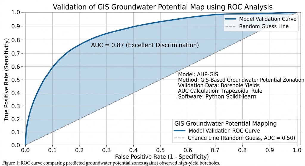
Groundwater potential studies commonly evaluate their results against existing borehole locations and yield records, sometimes using statistical measures and Receiver Operating Characteristic (ROC) analysis.
Step 1: Prepare the borehole dataset
Collect available borehole records from water authorities, geological surveys, drilling reports, or other reliable sources.
Useful attributes include:
| Attribute | Purpose |
|---|---|
| Borehole ID | Unique identifier |
| Coordinates | Location for spatial comparison |
| Drilled depth | Context for the aquifer interval |
| Static water level | Indicates water-level conditions |
| Tested discharge or yield | Measures borehole productivity |
| Test date and duration | Helps interpret differences between records |
| Aquifer or lithology | Supports hydrogeological interpretation |
Use measured borehole yield wherever possible. A recorded water strike or the presence of groundwater does not necessarily indicate a productive well. Also, distinguish borehole yield from sustainable aquifer yield: long-term availability requires additional hydrogeological assessment.
Check coordinate accuracy, duplicate borehole records, missing yield values, and inconsistent units before analysis.
Step 2: Extract the mapped potential class at each borehole
In QGIS:
-
Load the borehole point layer and the classified groundwater potential raster.
-
Verify that the borehole coordinates are correct and that the points overlap the valid raster extent.
-
Open Processing Toolbox and search for Sample raster values.
-
Set the borehole points as the input point layer.
-
Select the classified groundwater potential raster.
-
Run the tool to append the raster value at each borehole location.
-
Export the resulting attribute table for statistical analysis if needed.
In ArcGIS Pro:
-
Load the borehole point layer and the groundwater potential raster.
-
Open Analysis → Tools.
-
Search for Extract Multi Values to Points or an appropriate raster sampling tool.
-
Select the borehole point layer and the potential-zone raster.
-
Run the tool and examine the extracted zone value.
The resulting table should contain both the measured borehole information and the groundwater potential class predicted at each location.
Step 3: Compare potential classes with observed yield
Group the boreholes into yield categories that reflect the study’s hydrogeological context. There is no universal discharge threshold that separates low-, moderate-, and high-yield wells in every aquifer.
An example validation table might look like this:
| Borehole yield category | Low-potential zones | Moderate-potential zones | High-potential zones |
|---|---|---|---|
| Low yield | 22 | 12 | 4 |
| Moderate yield | 10 | 18 | 12 |
| High yield | 3 | 11 | 28 |
Illustrative counts only. These values are not observed research results.
A model that performs well would generally be expected to place a greater proportion of high-yield boreholes in high-potential zones than in low-potential zones.
However, overlapping distributions are normal. A low-potential pixel may still contain a productive borehole because of local fractures, an unrepresented aquifer, or errors in the thematic input layers.
Step 4: Quantify model performance
For a more rigorous research study, use one or more of the following methods.
A. Proportion of high-yield boreholes in high-potential zones
Calculate the proportion of observed high-yield boreholes that fall inside mapped high-potential zones. This is an intuitive first check, but it does not measure the full classification performance.
B. Confusion matrix
Where both predicted and observed conditions can be defined categorically, calculate the number of correctly and incorrectly classified observations. Derive measures such as sensitivity, specificity, and overall accuracy where suitable for the sampling design.
C. ROC curve and Area Under the Curve (AUC)
When validating high-yield groundwater occurrence as a binary outcome, define positive observations—for example, boreholes meeting the study’s high-yield criterion—and negative observations from the remaining eligible sample.
Use the continuous GPI score to calculate an ROC curve and its AUC. An AUC of 0.5 indicates discrimination no better than random ranking under the evaluation design, while a value closer to 1 indicates stronger discrimination. A high AUC alone does not establish calibration, sustainable yield, or generalization to a different region.
Step 5: Protect the validation from bias
A common research weakness is assessing a model with the same boreholes that were used to select weights, choose rating thresholds, or tune the final map.
Where sufficient data are available:
-
Set aside independent borehole records for validation before tuning the model.
-
Where practical, use spatially separated training and validation groups to reduce the risk of overly optimistic results from nearby, correlated boreholes.
-
Record unsuccessful or low-yield boreholes as well as productive wells.
-
Examine whether records are clustered near roads, settlements, or areas with more drilling activity.
-
Test whether reasonable changes to criterion weights, class ratings, or raster resolution substantially alter the predicted zones.
If the map performs poorly, revisit the input data, the conceptual model, and the pairwise judgments. A passing AHP consistency ratio cannot compensate for inaccurate data or unsuitable hydrogeological assumptions.
5. Common methodological pitfalls
Before reporting the results, check for these frequent problems.
Treating the weights as universal. Rainfall may dominate in one region, while lithology and fractures may control groundwater occurrence in another. Justify the weights for the specific aquifer setting.
Using a single factor as a proxy for the entire groundwater system. Lineament density, drainage density, or rainfall alone does not establish groundwater availability. Interpret them alongside geological and hydrogeological evidence.
Confusing potential with recharge. A location with high groundwater potential may contain a productive aquifer without being a major present-day recharge area.
Misclassifying raster values. Categorical codes should not be treated as continuous measurements. Reclassification must encode the suitability associated with each class.
Ignoring missing data. A cell with incomplete input data should not be presented as confidently classified merely because the overlay produced an output.
Choosing arbitrary zone thresholds. Equal intervals, Natural Breaks, and quantiles can produce different patterns. Report the classification method and, where possible, test it against borehole observations.
Neglecting groundwater quality and sustainability. A high-yield location may still have unsuitable water quality or an unsustainable pumping rate. These require separate assessment.
6. Summary and key takeaways
The Groundwater Potential Mapping AHP GIS workflow brings together hydrogeological knowledge, spatial data, and multi-criteria decision analysis to identify locations that deserve further groundwater investigation.
The process follows six core stages:
-
Select the criteria: Compile lithology, LULC, drainage density, slope, rainfall, and lineament density.
-
Calculate AHP weights: Construct the pairwise comparison matrix, normalize it, and calculate the priority vector.
-
Check consistency: Calculate the maximum eigenvalue, Consistency Index, and Consistency Ratio. Confirm that \(CR<0.10\).
-
Prepare raster layers: Reclassify all criteria to a common 1–5 suitability scale and align them spatially.
-
Apply weighted overlay: Multiply each standardized raster by its AHP weight and sum the results to create the groundwater potential index.
-
Validate the output: Compare mapped zones with observed borehole yield and, where data permit, use independent statistical validation.
The most important research principle is that AHP provides a transparent weighting framework, while the quality of the groundwater potential map depends on the quality of the underlying hydrogeological evidence, spatial data, suitability ratings, and validation.
A well-documented GIS-based groundwater potential map can help prioritize field surveys, geophysical investigations, and borehole exploration. It should inform those decisions rather than replace them.
Further reading and technical documentation
-
Groundwater potential mapping methodology: AHP-based groundwater potential mapping in the Buffalo catchment, South Africa — a published example of factor weighting and borehole-yield validation.
-
AHP and groundwater recharge research: Systematic review of GIS and multi-criteria decision analysis for groundwater recharge potential — reviews the use of spatial criteria and weighting approaches.
-
QGIS reclassification: QGIS raster analysis documentation — reference for reclassifying raster values using tables.
-
ArcGIS Pro weighted overlay: How Weighted Overlay works — describes the common evaluation scale, criterion influences, and raster combination process.