Spatial Lag vs. Spatial Error Models: Choosing the Right Spatial Econometric Model

 

1. Introduction: Why Standard OLS Regression Can Fail in Spatial Analysis

Imagine a researcher studying why property prices differ across neighborhoods. The researcher collects data on house prices, household income, distance to the city center, and access to public transportation. Using Ordinary Least Squares (OLS) regression, they estimate how these variables relate to property prices.

However, the resulting model leaves an important question unanswered: does the value of a house depend partly on the values of nearby houses, or are nearby properties similar because they share unmeasured characteristics?

This question lies at the heart of spatial econometrics.

Traditional OLS regression assumes that, after accounting for the explanatory variables, observations satisfy the relevant independence and error assumptions. In geographical datasets, this assumption may be violated because nearby locations often share characteristics, interact with one another, or experience similar unobserved conditions.

This phenomenon is known as spatial dependence, commonly investigated through measures of spatial autocorrelation.

For example, neighboring neighborhoods may have similar property prices because of shared schools and transport networks. Alternatively, they may experience similar prices because the model omits a geographically clustered factor, such as local development pressure.

These situations represent different spatial processes and may require different regression models.

Two widely used approaches are:

• Spatial Lag Model (SLM): Models spatial dependence in the dependent variable itself.
• Spatial Error Model (SEM): Models spatial dependence in the regression error term.

Understanding the difference is essential when choosing an appropriate spatial regression model in GIS.

1.1 Why Spatial Dependence Matters

OLS estimates a conventional linear regression:

[
Y=X\beta+\varepsilon
]

Where:

• (Y) is the dependent variable being explained.
• (X) represents the explanatory variables.
• (\beta) contains the regression coefficients.
• (\varepsilon) represents unexplained variation.

For example, (Y) might represent average neighborhood property prices, while (X) contains household income, accessibility, and population density.

Spatial dependence can affect this model in different ways.

When the dependent variable has spatial spillovers, neighboring values help determine the value at a particular location. If this process is ignored, OLS generally produces inconsistent coefficient estimates because the omitted spatially lagged dependent variable is endogenous.

When the error term is spatially correlated, nearby areas share unexplained influences. Under exogeneity, OLS coefficients can remain unbiased and consistent, but OLS is generally inefficient and conventional standard errors and hypothesis tests may be unreliable. If omitted factors are correlated with the explanatory variables, coefficient bias can also occur.

The key point is that spatial autocorrelation does not automatically mean OLS coefficients are biased. The consequences depend on the underlying spatial process.

2. Understanding the Spatial Weights Matrix

Before examining spatial lag and spatial error models, it is necessary to understand the spatial weights matrix, usually represented by (W).

This matrix describes which geographical observations are considered connected and how strongly they are weighted.

In GIS, neighboring areas can be defined using several approaches:

• Contiguity: Two polygon areas are neighbors if they share a boundary or a boundary point.
• Distance-based neighbors: Two locations are connected if they fall within a specified distance.
• K-nearest neighbors: Each location is connected to a specified number of its nearest neighbors.

For example, a city district might be connected to all districts sharing its boundary. The corresponding row in (W) identifies those neighbors, while other districts receive zero weights.

A row-standardized matrix converts each nonempty row’s weights to sum to one. Under this convention, (WY) can be interpreted as the weighted average of neighboring outcome values.

The chosen weights matrix matters because changing the definition of a neighbor can change the estimated spatial dependence. Analysts should therefore justify their choice using the study’s geography and substantive question.

3. Spatial Lag Model (SLM) Explained

The Spatial Lag Model, also known as the spatial autoregressive lag model or SAR lag model, is appropriate when the dependent variable in one location is influenced by the dependent variable in neighboring locations.

3.1 The Spatial Lag Model Formula

The model can be written as:

[
Y=\rho WY+X\beta+\varepsilon
]

Where:

• (Y) is the dependent variable.
• (WY) is the spatially lagged dependent variable.
• (\rho) is the spatial autoregressive coefficient.
• (X\beta) represents the effect of the explanatory variables.
• (\varepsilon) is the remaining error term.

The main addition to OLS is the term (\rho WY).

Instead of explaining an area’s outcome solely through its own characteristics, the model allows outcomes in neighboring areas to participate in the process.

3.2 What Does the Spatial Lag Coefficient Mean?

The coefficient (\rho) indicates the strength and direction of spatial dependence under the specified weights matrix.

When (\rho) is positive, higher neighboring outcomes are associated with higher outcomes in the focal location through the modeled spatial feedback mechanism. When it is negative, the modeled dependence operates in the opposite direction.

The precise interpretation depends on the model assumptions and spatial weights.

A significant (\rho) supports the presence of a spatial lag process, but it does not by itself establish a causal mechanism.

3.3 Practical Example: Neighborhood Housing Prices

Consider a property valuation study in which the dependent variable is average house price by neighborhood.

Suppose the following factors are included in the regression:

• Household income
• Distance to the central business district
• Access to public transport
• Housing density

Even after accounting for these characteristics, property prices may remain spatially interdependent.

Buyers compare nearby properties, valuations use neighboring sales as reference points, and demand in one neighborhood may influence demand in surrounding areas.

If the researcher has a defensible reason to believe that nearby property values influence local values, a spatial lag model may be appropriate.

The spatial lag term captures this dependence rather than treating every neighborhood’s outcome as completely independent of the others.

However, geographical similarity alone is not proof of direct spillovers. Shared amenities, omitted variables, and common market conditions can also generate spatial patterns.

3.4 Practical Example: Crime Rates

Suppose a researcher investigates crime rates across neighboring urban districts.

Crime patterns may be related across district boundaries because people move between areas, police patrols shift across nearby districts, or crime opportunities extend across administrative boundaries.

A spatial lag model may be suitable if the research hypothesis involves dependence in the crime outcome itself.

Yet crime clusters can also result from unmeasured socioeconomic conditions or differences in reporting practices. Researchers should distinguish a genuine outcome-interaction hypothesis from spatially clustered omitted factors.

3.5 Important Interpretation Warning

The coefficient (\rho) is not necessarily the complete marginal effect of a change in a predictor.

Because outcomes interact through the spatial system, a change in one location can affect its neighbors and potentially feed back to the original location. Researchers often calculate direct, indirect, and total impacts to describe these relationships more fully.

For further technical information, see the spatialreg documentation for spatial autoregressive models.

4. Spatial Error Model (SEM) Explained

The Spatial Error Model is used when unexplained influences are spatially correlated.

Unlike the spatial lag model, the SEM does not directly introduce neighboring values of the dependent variable into the regression equation. Instead, it models the spatial structure of the error term.

4.1 The Spatial Error Model Formula

The SEM is written as:

[
Y=X\beta+u
]

With the spatial error process:

[
u=\lambda Wu+\varepsilon
]

Where:

• (Y) is the dependent variable.
• (X\beta) represents the explanatory variables.
• (u) is the spatially structured error term.
• (\lambda) is the spatial error coefficient.
• (Wu) represents spatial dependence among the error terms.
• (\varepsilon) is the remaining disturbance, usually assumed to satisfy the model’s required independence conditions.

The key parameter is (\lambda).

If (\lambda) is nonzero, the model allows unexplained influences in nearby locations to be spatially related.

This does not mean the researcher knows exactly which missing factor caused the dependence. Rather, the model accounts for a specified spatial pattern in the unexplained component.

4.2 Practical Example: Crop Yield and Climate

Imagine a researcher examining crop yields across neighboring agricultural districts.

The model includes:

• Rainfall
• Average temperature
• Fertilizer application
• Irrigation availability

However, crop yields may still vary across the region because the dataset does not adequately capture every relevant condition.

Potential omitted influences include soil characteristics, localized pest pressure, terrain, and unmeasured farming practices.

Several of these factors may be spatially clustered. Neighboring farms often share similar soil conditions and local weather patterns.

If the remaining unexplained variation displays spatial dependence, an SEM may be appropriate.

The error component accounts for that dependence without assuming that one district’s crop yield directly determines the crop yield of another district.

4.3 Practical Example: Environmental Pollution

Consider a study estimating the relationship between industrial activity and air pollution.

The regression includes industrial density, traffic intensity, and population density. However, pollution levels may also depend on spatially patterned influences such as local meteorology, terrain, or unmeasured emission sources.

If these omitted influences produce spatial correlation in the regression errors, a spatial error model can help account for the remaining dependence.

Nevertheless, researchers should still seek relevant omitted variables where possible. An SEM does not identify missing variables automatically, and it does not replace sound scientific reasoning about the environmental process.

4.4 What Does the Spatial Error Coefficient Mean?

The coefficient (\lambda) describes the strength and direction of the spatial error process under the chosen weights matrix.

A statistically significant estimate can indicate that unexplained influences exhibit spatial dependence.

Unlike the spatial lag coefficient, however, (\lambda) is not interpreted as the direct influence of neighboring dependent-variable values.

That distinction is central to choosing the appropriate model.

5.  Spatial Lag vs Spatial Error Models: The Core Difference

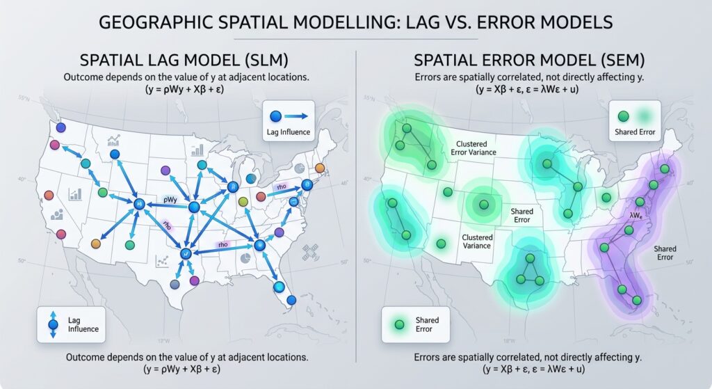
The difference becomes easier to remember when expressed as two questions.

Spatial Lag Model: Does the outcome in one location depend on outcomes in neighboring locations?

Spatial Error Model: Are the unexplained influences in nearby locations correlated?

Consider two neighborhoods with similar property prices.

Under the spatial lag explanation, the model allows surrounding property values to contribute to the outcome through a spatial feedback process.

Under the spatial error explanation, the neighborhoods may have similar prices because they share geographically clustered influences that the model does not fully capture.

These explanations can sometimes coexist. They should not be treated as mutually exclusive descriptions of every real-world spatial process.

6. Decision Framework: Using the Lagrange Multiplier Test

How can an analyst decide which model to use?

A common starting point is the Lagrange Multiplier (LM) diagnostic test, applied after estimating an OLS model and constructing an appropriate spatial weights matrix.

These diagnostics test whether a spatial lag or spatial error term is supported by the regression data.

The classical tests are useful for identifying candidate models, while their robust counterparts are particularly valuable when both classical tests are significant.

6.1 Step 1: Estimate the OLS Model

Begin with a conventional regression representing your research question.

For example:

[
Price_i=\beta_0+\beta_1Income_i+\beta_2Access_i+\varepsilon_i
]

Here, property price is the dependent variable, while income and accessibility are explanatory variables.

Before proceeding, check the model specification, explanatory variables, missing observations, and other standard regression diagnostics.

6.2 Step 2: Define the Spatial Weights Matrix

Create a spatial weights matrix using a defensible geographical relationship.

For instance, a neighborhood-level study could use contiguity weights based on polygon boundaries. A point-based study might use distance-based or nearest-neighbor weights.

Document the matrix construction, including any row standardization. The LM test results are conditional on the chosen spatial structure.

6.3 Step 3: Run the Classical LM Tests

Two key diagnostics are:

• LM-Lag: Tests the null hypothesis that the spatial lag coefficient (\rho) is zero.
• LM-Error: Tests the null hypothesis that the spatial error coefficient (\lambda) is zero.

A small p-value provides evidence against the corresponding null hypothesis, conditional on the test assumptions.

For instance, at a preselected significance level of 0.05, a p-value below 0.05 indicates that the tested null hypothesis is rejected.

However, classical LM-Lag and LM-Error tests can both be significant when one form of spatial dependence is responsible for the apparent evidence of the other.

This is why analysts commonly examine the robust tests as well.

6.4 Step 4: Examine the Robust LM Tests

The robust diagnostics adjust each test for the potential presence of the alternative form of spatial dependence.

Robust LM-Lag tests for an omitted spatial lag while accounting for possible spatial error dependence.

Robust LM-Error tests for spatial error dependence while accounting for a possible omitted spatial lag.

These tests are especially useful when both classical LM tests are significant.

The procedure follows the established spatial diagnostic framework associated with Anselin and colleagues. A detailed explanation is available in the PySAL specification testing documentation.

6.5 LM Diagnostic Decision Matrix

Classical LM-Lag	Classical LM-Error	Robust LM results	Suggested next step
Not significant	Not significant	Generally no evidence from these tests	Retain OLS as a candidate and investigate other diagnostics
Significant	Not significant	Robust lag supports the lag process	Consider the Spatial Lag Model
Not significant	Significant	Robust error supports the error process	Consider the Spatial Error Model
Significant	Significant	Only robust lag is significant	Prefer investigating the Spatial Lag Model
Significant	Significant	Only robust error is significant	Prefer investigating the Spatial Error Model
Significant	Significant	Both robust tests are significant	Consider a more general spatial model and investigate misspecification
Significant	Significant	Neither robust test is significant	Re-examine specification, weights, sample characteristics, and model assumptions

This matrix is a diagnostic guide rather than an automatic model-selection rule. The analyst should also consider economic theory, the study objective, residual diagnostics, and the behavior of the fitted models.

When both robust tests remain significant, a model incorporating both spatial lag and spatial error dependence, such as a SARAR/SAC model, may be worth investigating. A spatial Durbin model may also be appropriate when neighboring explanatory variables are substantively relevant.

When neither robust test is significant, that does not prove that OLS is correct. Other forms of dependence, omitted variables, heteroskedasticity, nonlinear relationships, or an unsuitable weights matrix may still require attention.

7. Practical Implementation in R

R provides the spdep and spatialreg packages for spatial diagnostics and spatial regression estimation.

The following example assumes that you have a polygon dataset named regions, with one row per region and numeric columns price, income, and access.

Step 1: Install and Load the Packages

install.packages(c("sf", "spdep", "spatialreg"))

library(sf)
library(spdep)
library(spatialreg)

Step 2: Create the Spatial Weights

# regions is an sf polygon object.
neighbors <- poly2nb(regions, queen = TRUE)

weights <- nb2listw(
  neighbors,
  style = "W",
  zero.policy = TRUE
)

Queen contiguity treats polygons that share a boundary or a vertex as neighbors. The row-standardized weights make the weights for each nonempty neighborhood sum to one.

zero.policy = TRUE permits regions without neighbors, but you must still inspect such regions and determine whether this treatment is substantively appropriate.

Step 3: Fit the OLS Model

ols_model <- lm(
  price ~ income + access,
  data = regions
)

summary(ols_model)

This estimates the baseline relationship between property price, income, and accessibility.

Step 4: Run the Spatial Diagnostics

lm_results <- lm.RStests(
  ols_model,
  listw = weights,
  test = "all"
)

summary(lm_results)

The lm.RStests() function reports the modern Rao’s score versions of the diagnostics, closely related to the traditional LM tests. In current versions of spdep, the names commonly include RSlag, RSerr, adjRSlag, and adjRSerr.

The robust tests correspond to adjRSlag and adjRSerr. Their p-values help assess which spatial dependence mechanism is supported after accounting for the competing form.

See the spdep diagnostic function documentation.

Step 5: Estimate the Candidate Spatial Model

If diagnostics and theory support a spatial lag model:

lag_model <- lagsarlm(
  price ~ income + access,
  data = regions,
  listw = weights,
  zero.policy = TRUE
)

summary(lag_model)

If they support a spatial error model:

error_model <- errorsarlm(
  price ~ income + access,
  data = regions,
  listw = weights,
  zero.policy = TRUE
)

summary(error_model)

Compare model diagnostics and fit, inspect residual spatial autocorrelation, and check whether conclusions remain stable under defensible alternatives for the weights matrix. Do not choose a model solely because it has the largest pseudo-(R^2).

The lagsarlm() and errorsarlm() functions are documented in spatialreg.

8. Which GIS Software Should You Use?

Spatial econometric modeling can be carried out in desktop software or a programming environment. The best option depends on your workflow, reproducibility requirements, and the complexity of the model.

Software	Main role	Spatial diagnostic and modeling options	Best suited to
GeoDa	Interactive exploratory spatial data analysis	OLS regression diagnostics, LM tests, spatial lag and spatial error estimation	Students learning spatial econometrics through a graphical interface
R: spdep + spatialreg	Statistical testing and model estimation	Classical and robust spatial diagnostics, SAR lag, SEM, and more general spatial regression models	Reproducible research and detailed statistical analysis
Python: PySAL spreg	Script-based spatial econometric analysis	OLS diagnostics, LM-Lag and LM-Error, robust LM tests, spatial lag and error estimation	Analysts integrating spatial regression into Python and GIS data-science workflows

GeoDa

GeoDa is a good starting point for students who want to explore spatial relationships interactively. You can prepare a spatial weights matrix, estimate an OLS regression, inspect spatial diagnostics, and estimate spatial lag or spatial error models.

The GeoDa Workbook provides practical exercises for spatial regression analysis.

R

R is particularly useful for transparent, reproducible workflows. The spdep package supports spatial diagnostics, while spatialreg estimates the spatial lag and spatial error models, among other specifications.

Python

Python is useful when spatial econometrics forms part of a larger data-processing or modeling pipeline. The PySAL spreg module supports OLS diagnostics and spatial regression estimation.

For example, its OLS documentation describes the available LM and robust LM diagnostics, while its API reference lists the available spatial regression estimators.

9. Summary Comparison Table

Feature	Spatial Lag Model (SLM)	Spatial Error Model (SEM)
Model formula	(Y=\rho WY+X\beta+\varepsilon)	(Y=X\beta+u,\quad u=\lambda Wu+\varepsilon)
Underlying spatial process	Dependence in the dependent variable	Dependence in unexplained influences
Key coefficient	(\rho), spatial lag coefficient	(\lambda), spatial error coefficient
Main question	Do neighboring outcomes participate in the process generating local outcomes?	Are unexplained factors spatially correlated?
Example	Property-price spillovers across neighborhoods	Crop yields affected by spatially clustered omitted soil or climate factors
Initial diagnostic	Classical LM-Lag	Classical LM-Error
Diagnostic when both classical tests are significant	Robust LM-Lag	Robust LM-Error
Recommended software	GeoDa, R spatialreg, Python PySAL	GeoDa, R spatialreg, Python PySAL

10. Student Takeaways

The difference between a spatial lag model and a spatial error model is not simply a matter of choosing the regression with the better fit. The models represent different explanations for spatial dependence.

A Spatial Lag Model is appropriate when the dependent variable itself follows a spatial interaction or feedback process. A Spatial Error Model is appropriate when unobserved influences remain spatially correlated.

The Lagrange Multiplier diagnostic framework helps distinguish these explanations by testing for spatial lag and spatial error dependence after estimating OLS. When both classical tests are significant, the robust versions offer a more informative starting point for model selection.

For a university GIS assignment, a strong analysis should document the spatial weights matrix, explain the theoretical reason for selecting a model, report the relevant LM diagnostics, estimate the supported candidate model, and check residual behavior afterward.

The central lesson is simple: Choose a Spatial Lag Model when the spatial process belongs in the outcome equation; choose a Spatial Error Model when it belongs in the error structure. Use diagnostics to inform that decision, but let the research question and the underlying geographical process guide the final specification.