Spatial Autocorrelation (Global Moran’s I) in GIS: Interpretation Guide

1. Introduction: Why Does Location Matter?

Imagine mapping malaria incidence across several districts. Some districts report high incidence, while others report low incidence. When the high-incidence districts are located near one another, the pattern may indicate spatial clustering. If neighbouring districts have contrasting incidence levels, the pattern may be more dispersed.

Traditional GIS mapping combined with tools for Global Morans I Spatial Autocorrelation GIS can reveal these patterns visually.However, a map alone cannot tell you whether the observed arrangement is statistically distinguishable from a random pattern.

This is where spatial autocorrelation—as well as programmatic approaches like vector data analysis using Python—becomes useful.

Understanding Tobler’s First Law of Geography

Geographer Waldo Tobler formulated the principle commonly known as the First Law of Geography:

“Everything is related to everything else, but near things are more related than distant things.”

In simple terms, places close to one another often share characteristics because they interact with similar environmental, social, economic, or physical processes.

Consider these examples:

• Housing prices: Neighbouring properties may have similar prices because they share access to transport, schools, and public services.
• Vegetation: Adjacent areas may have similar vegetation conditions because they experience comparable rainfall, soils, and land management.
• Public health: Nearby communities may experience similar disease patterns due to shared environmental conditions or connected populations.

However, nearby places are not always similar. A wealthy neighbourhood may sit next to a low-income settlement, or a healthy forest patch may border degraded land.

Spatial autocorrelation provides statistical tools for investigating whether geographic values tend to be similar or dissimilar among neighbouring locations.

One of the most widely used measures is Global Moran’s I, which summarizes the overall spatial autocorrelation of a numerical attribute across a study area. It is available in GIS software such as ArcGIS Pro and through open-source spatial statistics libraries.

2. What Is Global Moran’s I?

Global Moran’s I is a statistical measure that evaluates whether similar or contrasting attribute values are spatially associated across a dataset.

Unlike a simple average or standard deviation, Moran’s I considers both the attribute values and the spatial relationships between features.

For example, suppose you have population density values for 100 administrative wards. Global Moran’s I examines whether wards with high population density tend to be near other high-density wards, whether low-density wards tend to be near other low-density wards, or whether neighbouring wards tend to have contrasting values.

The method requires two main inputs:

1. A numeric attribute, such as population density, household income, rainfall, or disease incidence.
2. A spatial weights matrix describing which features are neighbours and how strongly they influence one another in the analysis.

The result is a single statistic describing the overall spatial pattern. The underlying principle and its interpretation are documented in the ArcGIS Pro Global Moran’s I guide.

The three broad spatial patterns

<box gap={3}> <row align=start gap={3}> <AsyncImage query=”GIS choropleth illustration spatial clustering high value polygons grouped together low value polygons grouped together” aspectRatio=”4:3″ width=”124px”/> <box flex=”1″ gap={1}> **1. Clustered pattern — positive spatial autocorrelation**

  Similar values tend to occur near one another. High values may form clusters of high values, while low values may form clusters of low values.

  <text color="secondary" size="sm">Example: Wards with high rental prices are concentrated around the same commercial centre.</text>
</box>

</row> <divider color=”subtle”/> <row align=start gap={3}> <AsyncImage query=”GIS choropleth illustration spatial dispersion alternating high low value polygons checkerboard pattern” aspectRatio=”4:3″ width=”124px”/> <box flex=”1″ gap={1}> **2. Dispersed pattern — negative spatial autocorrelation**

  Neighbouring features tend to have contrasting values. High values are more likely to occur near low values than near other high values.

  <text color="secondary" size="sm">Example: An alternating pattern of high- and low-value observations across neighbouring areas.</text>
</box>

</row> <divider color=”subtle”/> <row align=start gap={3}> <AsyncImage query=”GIS choropleth illustration random spatial pattern mixed high medium low value polygons” aspectRatio=”4:3″ width=”124px”/> <box flex=”1″ gap={1}> **3. Random pattern — no statistically detectable spatial autocorrelation**

  The observed arrangement does not provide sufficient statistical evidence of an overall spatial relationship under the selected model.

  <text color="secondary" size="sm">Example: High and low observations are distributed without a statistically significant overall clustering or dispersion pattern.</text>
</box>

</row> </box>

These categories describe the overall tendency of the data. They do not mean every individual feature follows the same pattern.

A dataset can contain a high-value cluster in one region and a low-value cluster elsewhere while still producing one global statistic.

Important: A nonsignificant Moran’s I does not prove that the data are genuinely random. It means the analysis has not found sufficient evidence to reject the null hypothesis of spatial randomness under the chosen spatial weights and statistical assumptions.

3. Understanding the Key Outputs

The Global Moran’s I tool in ArcGIS Pro reports five principal outputs:

Output	What it measures	Question it helps answer
Moran’s I Index	Direction and overall strength of spatial autocorrelation	Are similar or contrasting values spatially associated?
Expected Index	The expected value under the null hypothesis	What index would be expected under spatial randomness?
Variance	The statistical variability of the index under the null model	How much variation in Moran’s I is expected by chance?
Z-score	Standardized difference between the observed and expected index	How far is the result from the null expectation?
P-value	Evidence against the null hypothesis	Is the observed pattern statistically significant?

The five outputs are described in the official Spatial Autocorrelation tool documentation.

3.1 Moran’s I Index: From −1 to +1

The Moran’s I Index is the most recognizable output.

Its general interpretation is:

Index value	General interpretation
Close to +1	Strong positive spatial autocorrelation
Positive	Similar values tend to be near one another
Close to 0	Little overall spatial autocorrelation relative to the reference expectation
Negative	Neighbouring values tend to contrast
Close to −1	Strong negative spatial autocorrelation

In common row-standardized implementations, Moran’s I falls between −1 and +1. Its exact attainable range depends on the data and the spatial weights structure; without row standardization, some implementations can produce values outside that interval.

Suppose a study of household income produces a Moran’s I of +0.62. This indicates a substantial positive tendency for similar income values to be spatially associated.

However, the value alone does not establish statistical significance. A positive index may not be significantly different from its expected value. You must also examine the Z-score and P-value.

Likewise, a Moran’s I of −0.35 suggests spatial contrasts among neighbours, but the statistical significance of that pattern still needs to be assessed.

3.2 Expected Index: What Would Randomness Look Like?

The Expected Index is the theoretical Moran’s I value under the selected null hypothesis.

Under the standard randomization null model, the expected value is commonly expressed as:

[
E[I]=-\frac{1}{n-1}
]

Here, (n) is the number of spatial features.

For a dataset containing 101 wards, the expected value would be approximately −0.01.

This is important because the expected index is not necessarily exactly zero. For a finite dataset, it is commonly a small negative value under the standard formulation.

Practical interpretation: Compare the observed Moran’s I with the expected index rather than treating zero as the exact reference point in every analysis.

If the observed index is substantially higher than its expectation, the result points toward positive spatial autocorrelation. If it is substantially lower, the result points toward negative spatial autocorrelation. Statistical testing determines whether the difference is sufficiently large to reject the null hypothesis.

3.3 Variance: How Much Variation Is Expected by Chance?

The variance measures the statistical variability of Moran’s I under the null model.

It helps determine whether the difference between the observed and expected index is large relative to the amount of variation anticipated under the statistical assumptions.

Variance is not a separate measure of geographic clustering. It is part of the calculation used to assess the statistical significance of the observed index.

A useful way to think about it is to compare two research studies:

• Study A has an observed index only slightly above its expected value.
• Study B has a similar observed difference, but the null distribution is much less variable.

The second study may produce stronger statistical evidence against the null hypothesis, depending on the resulting standardized statistic.

3.4 Z-score: How Unusual Is the Result?

The Z-score expresses the difference between the observed Moran’s I and its expected value in standardized units.

Conceptually:

[
Z=\frac{I-E[I]}{\sqrt{\operatorname{Var}(I)}}
]

You do not normally need to calculate this manually when using a GIS tool because it is calculated as part of the analysis.

The interpretation is straightforward:

• A large positive Z-score indicates that the observed index is above the null expectation.
• A large negative Z-score indicates that it is below the null expectation.
• A Z-score near zero indicates that it is close to the null expectation relative to the estimated variability.

A positive Z-score is not a measure of the number of high-value locations. It describes the direction and statistical strength of the overall spatial autocorrelation relative to the null expectation.

3.5 P-value: Is the Pattern Statistically Significant?

The P-value measures how incompatible the observed result is with the null hypothesis, given the statistical test being used.

For Global Moran’s I, the usual null hypothesis is that the attribute values are spatially uncorrelated under the specified spatial relationships.

A smaller P-value provides stronger evidence against that null hypothesis.

P-value	Typical decision at a 5% significance level
Less than 0.01	Statistically significant at the 1% level
0.01 to less than 0.05	Statistically significant at the 5% level
0.05 or greater	Not statistically significant at the 5% level

These are conventional thresholds, not universal laws. Choose the significance level before interpreting the results.

A P-value of 0.03 does not mean there is a 3% probability that the null hypothesis is true. It means that, assuming the null hypothesis and statistical assumptions hold, a result at least as extreme as the observed result would have a probability of about 3% under the relevant test.

For a conventional two-sided normal approximation, absolute Z-scores of approximately 1.96 correspond to a 5% significance level, and 2.58 correspond to approximately 1%.

The direction of the pattern comes from the sign of the index and its deviation from expectation; the P-value helps determine whether there is enough evidence to make a statistical claim.

4. Step-by-Step Interpretation: Is the Pattern Significant?

Imagine that you are investigating whether population density is spatially clustered across administrative wards in a county.

Your Global Moran’s I analysis returns the following illustrative values:

Output	Illustrative result
Moran’s I Index	+0.27
Expected Index	−0.02
Variance	0.01
Z-score	+2.90
P-value	0.0037

These values are illustrative, not results from an actual dataset.

Step 1: Check the direction of Moran’s I

The observed index is +0.27, which is positive.

This suggests that wards with similar population density values tend to be located near one another.

Step 2: Compare the observed and expected index

The observed index, +0.27, is higher than the expected index, −0.02.

The positive difference indicates that the observed spatial association is more clustered than the null expectation.

Step 3: Read the Z-score

The Z-score is +2.90.

Under a normal approximation, this means that the observed statistic is nearly three standard errors above its expected value. This provides evidence against the null hypothesis in the direction of positive spatial autocorrelation.

Step 4: Check the P-value

The P-value is 0.0037, which is below 0.05 and also below 0.01.

Therefore, the observed global pattern is statistically significant at the 5% and 1% levels.

Step 5: State the conclusion carefully

A suitable interpretation for a university GIS report would be:

Global Moran’s I indicated statistically significant positive spatial autocorrelation in population density across the study area (I = 0.27, Z = 2.90, p = 0.0037). The results suggest that wards with similar population density values tend to be spatially associated under the selected spatial weights model.

This wording reports the direction, statistical significance, and interpretation without claiming that the result explains why population density is clustered.

What if Moran’s I is positive but P is 0.18?

In that case, the index points toward positive spatial autocorrelation, but the evidence would not be statistically significant at the 5% level.

You should report that the analysis did not find statistically significant overall spatial autocorrelation. You should not automatically claim that the pattern is random.

The result may be influenced by sample size, data variability, the number and arrangement of spatial features, or the chosen spatial weights matrix.

5. Spatial Conceptualization: Choosing a Spatial Weights Matrix

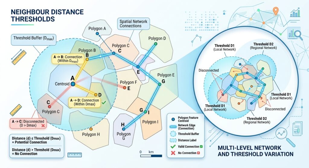
A spatial weights matrix defines the relationships among features in a spatial analysis.

Conceptually, imagine a square table in which every row and column represents a feature. Each entry indicates how strongly a feature is connected to another feature.

A weight of zero can indicate that two features are not treated as neighbours. A positive weight indicates that a spatial relationship exists, with the value specifying the strength of that relationship.

The matrix is central to Global Moran’s I because changing the definition of neighbourhood can change the statistical result. See the ArcGIS Pro spatial weights documentation.

5.1 Fixed Distance Band

A fixed distance band defines neighbours using a specified cutoff distance.

For example, if you choose a threshold of 5 kilometres, features within that distance of a target feature receive a weight of 1, while those outside it receive a weight of 0.

<box border radius=”lg” padding={3} gap={2}> <title size=”md”>Conceptual illustration: Fixed distance</title> <svg viewBox=”0 0 320 168″ width=”100%” xmlns=”http://www.w3.org/2000/svg“> <circle cx=”150″ cy=”78″ r=”54″ fill=”#3B82F6″ fillOpacity=”0.10″ stroke=”#3B82F6″ strokeWidth=”1.5″ strokeDasharray=”5 4″/> {#each [[150,78],[125,50],[180,44],[194,88],[130,106],[99,75],[220,42],[227,120],[65,113]] as p,i} <circle cx={p[0]} cy={p[1]} r={i===0?6:4.5} fill={i===0?”#2563EB”:(i<6?”#0F766E”:”#9CA3AF”)} stroke=”white” strokeWidth=”1″/> {/each} <text x=”159″ y=”95″ fill=”currentColor” fontSize=”10″>Target</text> <text x=”150″ y=”151″ fill=”currentColor” fontSize=”10″ textAnchor=”middle”>Inside threshold: weight 1</text> <text x=”150″ y=”164″ fill=”currentColor” fontSize=”10″ textAnchor=”middle”>Outside threshold: weight 0</text> </svg> <text color=”secondary” size=”sm”>Schematic only. The circle illustrates the distance threshold; point positions and distances are not to scale.</text> </box>

Advantages

• Easy to explain and communicate.
• All neighbours within the threshold receive equal weights.
• Useful when a realistic distance is known, such as a typical service area or ecological interaction distance.

Limitations

• Results can change substantially when the distance threshold changes.
• Dense areas may have many neighbours, while sparse areas may have very few.
• If the threshold is too small, some features may have no neighbours.

When to use it: Choose fixed distance when the research question involves a meaningful interaction scale and you can justify that scale using domain knowledge or supporting analysis.

For example, a study of access-related relationships among settlements might test a distance based on typical local travel distances, although straight-line distance does not necessarily represent actual road travel.

5.2 Inverse Distance Weights

Inverse distance weighting assigns greater influence to nearby features and lower influence to distant ones.

A common conceptual form is that weight decreases approximately with (1/d), where (d) is the distance between features. An inverse-distance-squared model decreases more rapidly, with a relationship proportional to (1/d^2).

The exact behaviour depends on the software settings, minimum-distance handling, and any specified distance threshold.

<box border radius=”lg” padding={3} gap={2}> <title size=”md”>Conceptual illustration: Inverse distance</title> <svg viewBox=”0 0 320 168″ width=”100%” xmlns=”http://www.w3.org/2000/svg“> <circle cx=”150″ cy=”78″ r=”6″ fill=”#2563EB”/> <line x1=”150″ y1=”78″ x2=”122″ y2=”52″ stroke=”#0F766E” strokeWidth=”3″/> <line x1=”150″ y1=”78″ x2=”183″ y2=”45″ stroke=”#0F766E” strokeWidth=”3″/> <line x1=”150″ y1=”78″ x2=”197″ y2=”87″ stroke=”#0F766E” strokeWidth=”3″/> <line x1=”150″ y1=”78″ x2=”99″ y2=”110″ stroke=”#0F766E” strokeWidth=”1.5″/> <line x1=”150″ y1=”78″ x2=”235″ y2=”116″ stroke=”#9CA3AF” strokeWidth=”1″ strokeDasharray=”4 4″/> {#each [[122,52],[183,45],[197,87],[99,110],[235,116]] as p,i} <circle cx={p[0]} cy={p[1]} r=”5″ fill={i<3?”#0F766E”:”#9CA3AF”}/> {/each} <text x=”160″ y=”95″ fill=”currentColor” fontSize=”10″>Target</text> <text x=”160″ y=”151″ fill=”currentColor” fontSize=”10″ textAnchor=”middle”>Near neighbours: greater weight</text> <text x=”160″ y=”164″ fill=”currentColor” fontSize=”10″ textAnchor=”middle”>Far neighbours: lower weight</text> </svg> <text color=”secondary” size=”sm”>Schematic only. Line thickness represents relative influence conceptually, not actual calculated weights.</text> </box>

Advantages

• Captures gradual differences in spatial influence.
• Avoids treating every neighbour within a large distance as equally influential.
• Can be appropriate when nearby features are expected to have stronger relationships than distant features.

Limitations

• The choice of inverse distance versus inverse distance squared changes the influence of nearby features.
• If no distance cutoff is specified in some GIS implementations, all features may be treated as neighbours, even very distant ones.
• Very small distances require careful handling, and a suitable projected coordinate system may be necessary.

When to use it: Consider inverse distance when the scientific reasoning suggests that spatial influence declines with distance rather than stopping abruptly at a boundary.

5.3 How do you choose a suitable weights matrix?

There is no universally correct spatial weights matrix. The choice should reflect the underlying process and the structure of the study data.

For a defensible thesis analysis:

1. Define the spatial relationship. Decide what makes two locations neighbours: distance, shared boundaries, travel networks, or another meaningful connection.
2. Check feature coverage. Ensure that your selected model does not leave features without neighbours unless that situation is explicitly handled.
3. Use appropriate distance units. Distance thresholds should be expressed in the units of the analysis coordinate system.
4. Test sensitivity. Where justified, compare more than one reasonable distance threshold or weighting scheme.
5. Document the final choice. Record the matrix type, threshold distance, standardization settings, and rationale.

For aggregated polygon data, row standardization is often recommended, especially when the number of neighbours differs across features. It adjusts the weights so that the influence of the neighbourhood is scaled relative to the total weight in each row.

The appropriate choice should be justified by the study design, not selected simply because it produces a statistically significant result.

6. When to Use Global vs. Local Moran’s I and Getis-Ord Gi*

Global Moran’s I summarizes the overall pattern across the entire study area. Sometimes that is enough to answer the research question. In other cases, you need to know exactly where clusters and outliers occur.

Three methods serve related but distinct purposes.

Method	Main question	Typical output
Global Moran’s I	Is there overall spatial autocorrelation?	One global statistic and significance test
Anselin Local Moran’s I	Where are local clusters and spatial outliers?	Local statistics and High–High, Low–Low, High–Low, Low–High classifications
Getis-Ord Gi*	Where are statistically significant concentrations of high or low values?	Hot spot and cold spot statistics

Global Moran’s I: Overall pattern

Use Global Moran’s I when your main question concerns the overall distribution of a variable across a study area.

For example: Is household income spatially clustered across all wards in the county?

The result tells you about the overall pattern, but it does not identify individual hot spots or outlier locations.

Anselin Local Moran’s I: Clusters and outliers

Local Moran’s I evaluates spatial autocorrelation for individual features in relation to their neighbours.

It can identify four important patterns:

• High–High (HH): A high-value feature surrounded by high-value neighbours.
• Low–Low (LL): A low-value feature surrounded by low-value neighbours.
• High–Low (HL): A high-value feature surrounded by low-value neighbours.
• Low–High (LH): A low-value feature surrounded by high-value neighbours.

For example, a regional income study might identify an affluent ward surrounded by lower-income wards. That feature could be a High–Low spatial outlier if the local statistic is significant.

The classifications should not be treated as meaningful unless the associated local tests and significance criteria support them.

Getis-Ord Gi*: Hot spots and cold spots

Getis-Ord Gi* focuses on identifying concentrations of high or low values in a spatial neighbourhood.

For example, a public health analyst may use it to locate areas with statistically significant concentrations of high reported disease rates, or an environmental researcher may use it to identify high-value vegetation index clusters.

Gi* is useful for hot spot and cold spot analysis, while Local Moran’s I additionally identifies local spatial outliers such as High–Low and Low–High patterns.

Important: When conducting Local Moran’s I or Gi* across hundreds of features, you perform many local significance tests. Consider an appropriate multiple-testing correction, where suitable, and report the method used. Do not interpret every individually significant result as reliable without considering the number of tests and the assumptions behind the analysis.

A practical decision rule

Use Global Moran’s I to answer:

Is spatial autocorrelation present overall?

Use Local Moran’s I to answer:

Where are the local clusters and contrasting spatial outliers?

Use Getis-Ord Gi* to answer:

Where are the statistically significant concentrations of high and low values?

These tools complement one another. For an academic study, it can be useful to begin with a global assessment and then conduct local analysis if the research question requires location-specific results.

7. Common Interpretation Mistakes

Before including the result in a GIS report or thesis, avoid these common errors.

Mistake 1: Interpreting Moran’s I without significance. A positive value does not automatically establish statistically significant clustering. Read the Z-score and P-value alongside the index.

Mistake 2: Treating a nonsignificant result as proof of randomness. Failure to reject the null hypothesis does not establish that spatial processes are random. It indicates insufficient evidence under the selected analytical model.

Mistake 3: Choosing an arbitrary distance threshold. An inappropriate spatial weights matrix can distort the interpretation. Justify the neighbourhood structure using substantive knowledge and appropriate sensitivity checks.

Mistake 4: Confusing spatial association with causation. Statistically significant autocorrelation does not explain why the observed pattern exists. Additional analysis is needed to investigate possible environmental, socioeconomic, or demographic explanations.

Mistake 5: Comparing Z-scores across unrelated study designs. Z-scores and P-values depend on the data, spatial weights, and analytical settings. Comparisons are meaningful only when the study designs and parameters are suitably comparable.

8. Conclusion

Global Moran’s I is a valuable tool for quantitative spatial analysis because it moves spatial pattern interpretation beyond visual inspection.

The Moran’s I Index describes the direction of overall spatial autocorrelation; the Expected Index provides the reference value under the null model; the Variance supports the statistical test; and the Z-score and P-value help determine whether the result is statistically significant.

The spatial weights matrix is equally important because it defines the neighbourhood relationships examined by the statistic. Fixed distance band and inverse distance weights represent different assumptions about how spatial influence operates.

For university GIS projects, a strong interpretation should report the index, expected index where relevant, Z-score, P-value, spatial weights choice, and study context. It should then explain what the results suggest without claiming to establish causation.

The most important principle is simple: Global Moran’s I tells you whether the overall spatial arrangement of values is consistent with spatial autocorrelation under a specified model—not why the pattern exists or exactly where every cluster occurs.

For further study, explore the official Global Moran’s I documentation, the spatial weights reference, and the Local Moran’s I guide.