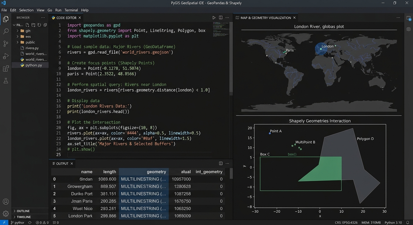
PyGIS Starter Guide: GeoPandas vs. Shapely for Vector Data Analysis

 

1. Introduction: Why Learn Open-Source Python GIS?

Using tools like GeoPandas vs Shapely PyGIS, traditional GIS applications such as QGIS and ArcGIS provide powerful frameworks for mapping, spatial analysis, and data management. However, when you need to repeat an analysis across hundreds of datasets, combine GIS with statistical models, or build a reproducible research workflow, programming offers additional flexibility.

This is where PyGIS, or open-source spatial programming with Python, becomes valuable. The Python geospatial ecosystem includes specialized libraries for working with vector data, raster imagery, coordinate systems, and spatial statistics. For visualizing your vector layouts, you can also check out this guide on how to export high-resolution vector PDFs and SVGs from GIS. includes specialized libraries for working with vector data, raster imagery, coordinate systems, and spatial statistics. The PyGIS learning resource provides tutorials covering many of these applications.

Two important libraries in this ecosystem are Shapely and GeoPandas. Although they are closely related, they solve different problems.

Shapely focuses on creating and analyzing individual geometric objects, such as points, lines, and polygons. GeoPandas builds on Python’s data-analysis ecosystem to manage entire spatial datasets, combine attribute tables with geometries, and perform operations such as spatial joins.

For example, imagine you are studying access to healthcare facilities in a county.

• Shapely can create a 500-metre buffer around a hospital and test whether another geometry intersects that buffer.
• GeoPandas can read hundreds of hospital locations and administrative boundaries, calculate buffers for every hospital, and join facilities to the administrative areas in which they are located.

Both operations involve geometry, but the scale and organization of the work are different.

This guide explains how each library works, provides practical Python examples, and shows how to combine them in a reproducible GIS workflow.

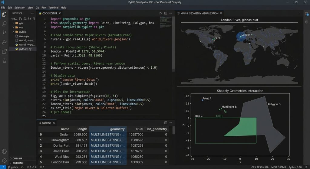
2. Understanding Shapely: Working with Individual Geometries

Shapely is an open-source Python library for constructing, manipulating, and analyzing planar geometric objects. It uses the GEOS geometry engine for core geometric operations. Its objects and methods support common tasks such as calculating distances, creating buffers, testing intersections, and combining shapes. See the Shapely user manual.

Think of Shapely as the geometry specialist within your Python GIS toolkit.

2.1 The three basic geometry types

Vector GIS data commonly represents real-world features using three fundamental geometry types.

Point: Represents a single coordinate location, such as a water sampling station or hospital.

from shapely.geometry import Point

hospital = Point(500000, 9850000)

print(hospital)
print(hospital.x)
print(hospital.y)

The coordinates in this example are illustrative. They represent an x-coordinate and a y-coordinate in a projected coordinate system, rather than longitude and latitude.

The Point() constructor creates the geometry. The .x and .y properties retrieve its coordinate values.

LineString: Represents a line defined by an ordered series of coordinates. Examples include roads, rivers, and hiking trails.

from shapely.geometry import LineString

river = LineString([
    (500000, 9850000),
    (501000, 9851000),
    (502500, 9851500)
])

print("Length:", river.length)

The LineString() constructor connects the supplied coordinates. Its .length property calculates the length in the geometry’s coordinate units.

Polygon: Represents an enclosed area, such as a forest reserve, agricultural field, or administrative boundary.

from shapely.geometry import Polygon

farm = Polygon([
    (500000, 9850000),
    (501000, 9850000),
    (501000, 9851000),
    (500000, 9851000),
    (500000, 9850000)
])

print("Area:", farm.area)

The coordinates trace the polygon boundary and return to the starting point to close the ring. The .area property calculates the planar area in squared coordinate units.

If the coordinates are measured in metres, the area is expressed in square metres.

2.2 Practical example: Creating a buffer around one point

A buffer is a polygon representing locations within a specified distance of a geometry.

Buffers are useful for studying questions such as:

• Which buildings lie within 500 metres of a road?
• What land falls within a monitoring zone around a river?
• Which homes are located near a public facility?

Consider a single sampling station. You want to create a 500-metre buffer around its location.

from shapely.geometry import Point

# Create a point using projected coordinates
station = Point(500000, 9850000)

# Create a 500-unit buffer
buffer_zone = station.buffer(500)

# Inspect the result
print("Geometry type:", buffer_zone.geom_type)
print("Area:", round(buffer_zone.area, 2))
print("Valid geometry:", buffer_zone.is_valid)

How the code works

1. Point(500000, 9850000) creates the sampling station.
2. .buffer(500) constructs a polygon extending 500 coordinate units around it.
3. .geom_type identifies the result as a polygon.
4. .area calculates its planar area.
5. .is_valid checks whether the geometry satisfies the geometry engine’s validity rules.

If the coordinate units are metres, the intended buffer radius is 500 metres. The theoretical area of a complete circle with that radius is approximately (785,398\text{ m}^2). Shapely represents circular arcs using line segments, so the calculated area is an approximation whose precision depends partly on the buffer settings.

An essential GIS warning: Shapely does not automatically understand coordinate reference systems. If you construct a point using longitude and latitude, buffer(500) does not create a 500-metre buffer. It uses 500 coordinate units, which would mean degrees for longitude-latitude coordinates. Use an appropriate projected coordinate system for planar distance and area calculations.

2.3 What else can Shapely do?

Beyond buffering, Shapely supports common geometric operations.

Operation	Example	Purpose
Distance	point_a.distance(point_b)	Measure planar distance
Intersection test	polygon.intersects(road)	Check whether geometries touch or overlap
Containment test	polygon.contains(point)	Test whether a geometry contains another
Area	polygon.area	Calculate planar area
Union	polygon_a.union(polygon_b)	Combine two geometries
Difference	polygon_a.difference(polygon_b)	Remove the portion occupied by another geometry
Buffer	point.buffer(500)	Create a distance-based polygon

These operations are particularly useful when you need direct control over geometry, are developing a custom spatial algorithm, or want to manipulate a small number of features without managing an entire GIS dataset.

However, Shapely by itself is not a replacement for a complete spatial table. It does not provide GeoPandas-style attribute-table management, integrated coordinate reference system handling, and convenient vector-file workflows.

That is where GeoPandas becomes useful.

3. Understanding GeoPandas: Managing Entire Spatial Datasets

GeoPandas extends the functionality of the pandas data-analysis library to spatial vector data. It introduces two central structures: the GeoSeries and the GeoDataFrame.

A GeoDataFrame combines the familiar rows and columns of a pandas DataFrame with a geometry column that stores Shapely objects. This makes it possible to filter records, analyze attributes, manipulate geometries, and combine spatial datasets using an integrated interface.

For a detailed introduction, see the GeoPandas documentation.

3.1 What is a GeoDataFrame?

Imagine an attribute table containing hospital locations.

hospital_id	name	beds	geometry
1	Hospital A	120	Point geometry
2	Hospital B	65	Point geometry
3	Hospital C	90	Point geometry

The first three columns store ordinary attributes. The geometry column stores the spatial representation of each hospital.

GeoPandas manages the table, while Shapely provides the geometric objects used for many spatial operations.

This combination allows you to perform normal data analysis and spatial analysis within the same workflow.

3.2 Installing GeoPandas

For a new student environment, installing GeoPandas through Conda and the conda-forge channel is a practical starting point because it manages the library’s geospatial dependencies.

In your terminal, run:

conda create -n pygis -c conda-forge geopandas jupyterlab
conda activate pygis

This creates an environment called pygis containing GeoPandas and JupyterLab. You can then start JupyterLab from that activated environment.

The official GeoPandas installation guide provides additional options, including pip installation.

3.3 Reading shapefiles and GeoJSON

GeoPandas uses read_file() to load spatial vector datasets into a GeoDataFrame. It supports formats such as ESRI Shapefile, GeoJSON, and GeoPackage through geospatial file-reading engines. See the read_file reference.

import geopandas as gpd

# Read a shapefile containing administrative boundaries
wards = gpd.read_file("data/wards.shp")

# Read a GeoJSON file containing hospital locations
hospitals = gpd.read_file("data/hospitals.geojson")

# Inspect the datasets
print(wards.head())
print(hospitals.head())

# Check their coordinate reference systems
print("Wards CRS:", wards.crs)
print("Hospitals CRS:", hospitals.crs)

Replace the file paths with the locations of your actual datasets.

The .head() method displays the first few records, helping you inspect field names and values. The .crs property identifies the coordinate reference system associated with each dataset, when that information is available.

You can also inspect the number of features:

print("Number of wards:", len(wards))
print("Number of hospitals:", len(hospitals))

This is an important first step before running spatial analysis. It helps confirm that the datasets loaded successfully and contain the expected number of records.

3.4 Practical example: Performing a spatial join

A spatial join links records from two datasets based on a geographic relationship instead of relying only on a shared attribute such as an identification number.

For example, suppose you have:

• A polygon dataset containing administrative wards.
• A point dataset containing hospital locations.

You want to determine which ward contains each hospital.

GeoPandas provides sjoin() for this purpose. It evaluates a spatial predicate, such as within or intersects, to match the geometries and combine their attributes. See the GeoPandas spatial joins guide.

import geopandas as gpd

# Load the input datasets
wards = gpd.read_file("data/wards.shp")
hospitals = gpd.read_file("data/hospitals.geojson")

# Confirm that both datasets have coordinate systems
if wards.crs is None or hospitals.crs is None:
    raise ValueError(
        "One or both datasets have no CRS. "
        "Verify the correct CRS before continuing."
    )

# Transform hospital coordinates to match the ward dataset
if hospitals.crs != wards.crs:
    hospitals = hospitals.to_crs(wards.crs)

# Keep only the ward fields needed in the output
ward_attributes = wards[["ward_name", "geometry"]]

# Match each hospital to the ward containing it
hospital_wards = gpd.sjoin(
    hospitals,
    ward_attributes,
    how="left",
    predicate="within"
)

# Inspect the results
print(hospital_wards.head())

# Save the result as a GeoPackage
hospital_wards.to_file(
    "outputs/hospitals_by_ward.gpkg",
    layer="hospital_wards",
    driver="GPKG"
)

This example assumes the ward attribute table contains a field named ward_name. Replace it with the actual field in your boundary dataset.

Understanding the important lines

1. Check the coordinate reference systems

A spatial join requires geometries to be represented in a compatible coordinate system. If one dataset has missing CRS information, determine its correct CRS from reliable metadata before proceeding.

2. Reproject the hospitals

hospitals = hospitals.to_crs(wards.crs)

This transforms the hospital coordinates into the ward dataset’s CRS. It is different from simply assigning a CRS label: reprojection changes the coordinate values to express the same locations in a different coordinate system.

3. Select the relevant ward attributes

ward_attributes = wards[["ward_name", "geometry"]]

This removes unnecessary columns from the right-hand dataset, keeping the result easier to inspect.

4. Run the spatial join

hospital_wards = gpd.sjoin(
    hospitals,
    ward_attributes,
    how="left",
    predicate="within"
)

The within predicate matches a hospital point to a ward polygon that contains it. The how="left" setting preserves all hospital records, including those that do not match a ward. Unmatched records will have missing values for the joined ward attributes.

Points lying exactly on polygon boundaries require special attention because within may not treat them as contained. Depending on the research question, another predicate may be more appropriate.

5. Export the output

to_file() writes the joined dataset to a GeoPackage. The output can then be opened in QGIS or another compatible GIS application for mapping, validation, and further analysis.

The spatial join is not just an attribute merge. It uses spatial relationships to determine which records belong together.

3.5 Other useful GeoPandas operations

GeoPandas provides many operations commonly encountered in GIS assignments.

# Select hospitals with more than 100 beds
large_hospitals = hospitals[hospitals["beds"] > 100]

# Create buffers for every hospital
# Use an appropriate projected CRS with metre units first.
hospital_buffers = hospitals.copy()
hospital_buffers["geometry"] = hospitals.geometry.buffer(500)

# Calculate polygon area
# Only use a suitable projected CRS and check its units.
wards["area_sq_units"] = wards.geometry.area

# Display a quick map
wards.plot()

These short examples demonstrate how GeoPandas combines table-based operations with geometry processing.

The buffer example assumes the input coordinates use a suitable projected CRS with metre units; otherwise, a distance of 500 will not represent 500 metres. Similarly, the polygon-area example reports squared coordinate units, which might be square metres, square feet, or another unit depending on the projection.

4. GeoPandas vs. Shapely: Key Differences

The main distinction is between managing spatial datasets and operating on geometries.

Feature	Shapely	GeoPandas
Primary purpose	Constructing and analyzing geometries	Managing and analyzing spatial tables
Main data structures	Point, LineString, Polygon, and other geometry types	GeoSeries and GeoDataFrame
Attribute tables	No integrated DataFrame structure	Supports pandas-style rows, columns, and filtering
Reading vector files	Not its main role	Supports reading and writing common vector formats
Spatial operations	Geometry-level operations	Dataset-level operations built around spatial geometries
Spatial joins	Supplies geometry predicates used in matching	Provides sjoin() for dataset joins
CRS management	Does not track or transform coordinate reference systems	Stores CRS information and supports reprojection
Performance	Efficient geometry processing; Shapely 2 provides vectorized operations	Efficient table-based workflows and spatial-index-assisted operations
Best use case	Custom geometry calculations or geometric algorithms	Analysis involving complete vector datasets
Typical output	A geometry, geometry array, or geometric result	A spatial table or processed geometry column

Which one is faster?

There is no universal winner.

For individual geometry calculations, Shapely offers the operations you need without requiring a GeoDataFrame. Shapely 2 also provides vectorized operations that can process arrays of geometries efficiently.

For dataset-wide operations, GeoPandas provides convenient column-based processing and uses spatial indexing to reduce unnecessary geometry comparisons in operations such as spatial joins and clipping.

The GeoPandas spatial indexing guide explains how spatial indexes improve the search for geometries that might satisfy a spatial relationship.

Actual performance depends on dataset size, geometry complexity, file-reading overhead, spatial indexing, and the operation being performed.

A useful rule is to choose the library based on the problem rather than assuming that one is inherently faster for every task.

5. How They Work Together: GeoPandas Uses Shapely

The relationship between the libraries is easiest to understand when you inspect the geometry column of a GeoDataFrame.

Consider this simple workflow:

import geopandas as gpd
from shapely.geometry import Point

# Create sample hospital locations
hospitals = gpd.GeoDataFrame(
    {
        "hospital": ["A", "B", "C"],
        "beds": [120, 65, 90],
        "geometry": [
            Point(500000, 9850000),
            Point(501000, 9851000),
            Point(502000, 9852000)
        ]
    },
    crs="EPSG:32737"
)

# Inspect the geometry objects
print(type(hospitals.geometry.iloc[0]))

# Buffer every hospital by 500 metres
buffers = hospitals.geometry.buffer(500)

# Store the buffers in a new GeoDataFrame
hospital_buffers = gpd.GeoDataFrame(
    hospitals[["hospital", "beds"]].copy(),
    geometry=buffers,
    crs=hospitals.crs
)

# Display the resulting data
print(hospital_buffers.head())

# Export the buffer polygons
hospital_buffers.to_file(
    "outputs/hospital_buffers.gpkg",
    layer="hospital_buffers",
    driver="GPKG"
)

This example uses illustrative coordinates. EPSG:32737 is a projected coordinate reference system with metre units; real coordinates should be verified against the actual study area and data source.

The workflow demonstrates how the two libraries cooperate.

First, Shapely’s Point() constructor creates the hospital geometries. GeoPandas stores them in the GeoDataFrame’s active geometry column alongside ordinary attributes such as hospital names and bed counts.

Next, hospitals.geometry.buffer(500) applies the geometry operation to the complete geometry column. GeoPandas exposes this operation through its geometry structures, while Shapely supplies the underlying geometric functionality.

The result is a collection of buffer polygons. GeoPandas then combines those polygons with the original hospital attributes and writes the resulting spatial table to a GeoPackage.

Conceptually, the workflow is:

Hospital coordinates and attributes
                |
                v
      Shapely Point objects
                |
                v
       GeoPandas GeoDataFrame
                |
                v
     GeoSeries.buffer(500)
                |
                v
 Shapely geometry processing
                |
                v
       Buffer polygons
                |
                v
     Output GeoDataFrame
                |
                v
       GeoPackage file

The diagram is conceptual rather than a complete description of every internal implementation step. GeoPandas manages the data structure and operation, while Shapely provides much of the vector geometry functionality.

This combination is powerful because you can use familiar pandas operations for attribute filtering and aggregation alongside geometric calculations.

6. Common Beginner Mistakes to Avoid

Mistake 1: Using latitude and longitude for metre-based buffers

A coordinate such as Point(36.8, -1.3) contains longitude and latitude values if the coordinate system is EPSG:4326. Calling .buffer(500) on that point does not create a 500-metre radius.

Solution: Reproject your dataset to an appropriate projected coordinate reference system before performing planar distance or area calculations.

Mistake 2: Confusing assigning a CRS with reprojecting data

set_crs() identifies the coordinate reference system associated with existing coordinates. to_crs() transforms coordinates from one CRS to another.

Solution: Verify the source data’s true CRS before assigning it. Use to_crs() when you need to transform coordinates. Consult the GeoPandas projections guide.

Mistake 3: Assuming a spatial join always returns one match per feature

A feature may match multiple polygons, or it may not match any polygon. The output depends on the spatial predicate and the spatial arrangement of the data.

Solution: Inspect unmatched records, investigate boundary cases, and confirm whether your analysis expects one-to-one, one-to-many, or unmatched relationships.

7. Conclusion: Which Library Should You Learn First?

Both GeoPandas and Shapely are fundamental tools for open-source Python GIS, and learning one does not eliminate the need for the other.

Start with Shapely to understand points, lines, polygons, spatial relationships, buffers, intersections, and geometric operations. These concepts build the foundation for computational geometry and help explain what GIS software does behind the scenes.

Move to GeoPandas when you need to manage actual vector datasets, work with attribute tables, read shapefiles and GeoJSON files, transform coordinate systems, and perform spatial joins across many features.

For university projects, you will often use both together. Shapely provides the geometric building blocks, while GeoPandas organizes those geometries into a spatial data-analysis workflow.

Suggested learning roadmap for students

Stage 1 — Python foundations: Learn variables, lists, dictionaries, loops, functions, and importing libraries.

Stage 2 — Shapely fundamentals: Create geometries and practise buffering, measuring distances, testing intersections, and combining polygons.

Stage 3 — GeoPandas essentials: Read a shapefile or GeoJSON dataset, inspect its fields, filter records, check its CRS, and export processed results.

Stage 4 — Dataset-level analysis: Perform spatial joins, clipping, dissolving, overlay operations, and geometry validation.

Stage 5 — Build a portfolio project: Use public road, health facility, or administrative boundary data to conduct a complete spatial analysis, document your methodology, and publish reproducible Python code.

The objective is to move beyond repeating GIS operations manually and develop workflows you can understand, explain, validate, and reuse.

By combining GeoPandas with Shapely, you gain a practical foundation for spatial data science, environmental analysis, transport accessibility studies, urban planning, and remote sensing support workflows.