Table of Contents

Demographic Analysis in GIS: 5 Steps to Map Census Data

Performing demographic analysis GIS allows you to turn census tables into meaningful maps showing population, income, age, housing, poverty, education, and other socioeconomic patterns. For university GIS assignments, however, the hardest part is often not the mapping itself—it is getting the tabular data to join correctly with geographic boundaries.

You may download a CSV or XLSX file containing census statistics, only to discover that your GEOID or FIPS codes have lost leading zeros, fields have different data types, or the table join produces unexpected NULL values.

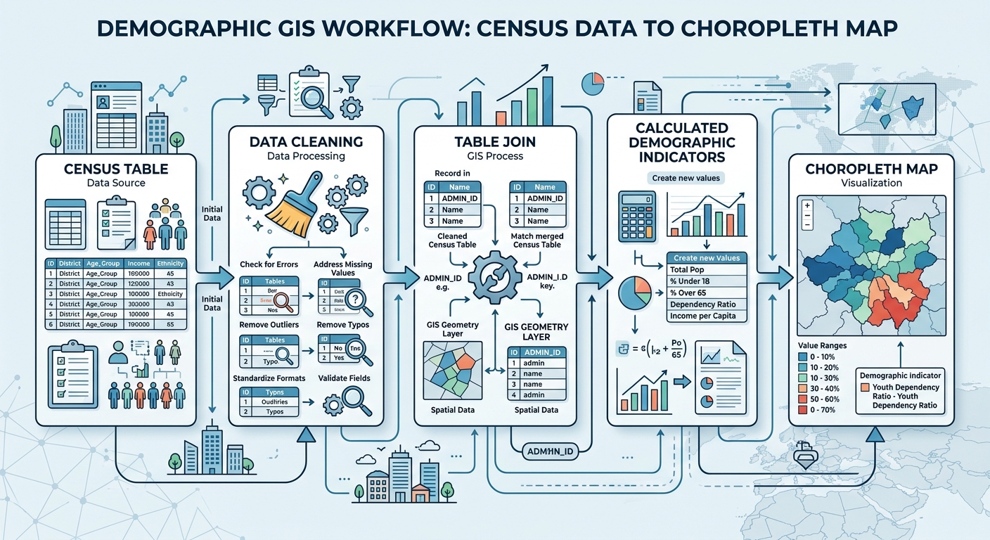
This guide presents a complete workflow from finding census data → cleaning identifiers → joining tables → calculating demographic indicators → creating and interpreting choropleth maps.

Demographic Analysis in GIS: The Complete Workflow

A reliable demographic mapping workflow follows five main stages:

Source census and boundary data
Clean and standardize identifier fields
Join demographic tables to geographic boundaries
Calculate meaningful demographic indicators
Create and interpret a choropleth map

The key principle is simple: your statistical table and spatial layer must share a reliable geographic identifier before you attempt the join.

Step 1: Source Census and Demographic Data

Before opening QGIS or ArcGIS Pro, determine exactly what demographic question your assignment is asking.

For example:

Where are population densities highest?
Which census tracts have the highest poverty rates?
Where is the elderly population concentrated?
How does median household income vary geographically?
Which areas have the highest percentage of children?

Your question determines which variables you need.

Use the U.S. Census Bureau

For U.S.-based assignments, the U.S. Census Bureau is one of the most important sources of demographic information.

[External Link Placeholder: U.S. Census Bureau data tools]

Depending on the assignment, you may encounter:

Decennial Census data
American Community Survey (ACS)
Population estimates
Housing statistics
Economic and socioeconomic variables

Census datasets are commonly available as CSV, XLSX, API responses, or other tabular formats.

Use NHGIS for Historical or Harmonized Data

The IPUMS National Historical Geographic Information System (NHGIS) is another useful source, particularly when an assignment requires historical census data or harmonized geographic information.

NHGIS can be particularly useful when you need to compare demographic characteristics across multiple census years.

Find Boundary Data

Your demographic table is not enough to create a map.

You also need a spatial boundary layer representing the geographic units in the table.

Examples include:

States
Counties
Census tracts
Block groups
ZIP Code Tabulation Areas
Municipal boundaries

The geographic level must match the demographic data.

For example, county-level statistics should be joined to county boundaries—not census tract boundaries.

Check the Geographic Identifier

Before downloading anything, identify the field that connects the table to the spatial layer.

Common identifiers include:

GEOID
FIPS code
State FIPS
County FIPS
Tract code
Block group code

The identifier is effectively the key that allows GIS to connect the two datasets.

Step 2: Clean Census Tables Before Joining

Data cleaning is one of the most important stages of demographic analysis GIS.

A table can look perfectly normal in Excel while still failing to join correctly in GIS.

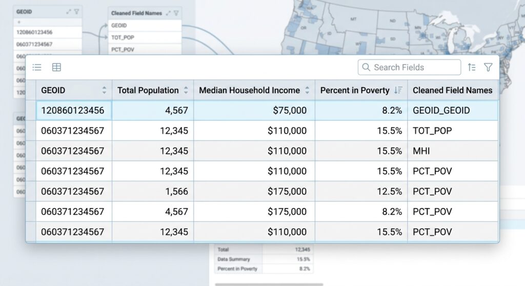
Inspect the Identifier Field

Suppose your census table contains:

GEOID	Population
01001	58,000
01003	220,000
01005	27,000

The GEOID must be treated consistently.

If one dataset stores 01001 as text but another stores it as a number, GIS may not recognize them as matching values.

Preserve Leading Zeros

This is one of the most common census-data problems.

A code such as:

01001

can accidentally become:

1001

when a CSV is opened in spreadsheet software or imported with automatic numeric type detection.

The two values are not equivalent as strings.

Pro Tip: Geographic identifiers should generally be treated as text/string fields, not numerical measurements.

If your identifier has five digits, make sure every record follows the same format.

Check Field Names

Clean confusing or excessively long field names before beginning the analysis.

For example:

B01001_001E

may represent a census variable that needs a more descriptive name such as:

Total_Pop

Keep the original variable definitions documented separately so that you can explain exactly what the field represents.

Check for Null Values

Look through your table for:

Blank GEOIDs
Missing demographic values
Duplicate identifiers
Invalid characters
Unexpected spaces
Different code formats

A single extra space can cause a join to fail.

For example:

01001

and

01001

may appear identical visually but can be treated differently by software.

Step 3: Join Census Data to GIS Boundaries

Once the table and boundary layer have compatible identifiers, you can perform the table join.

The basic relationship is:

Spatial boundary GEOID → Census table GEOID

The GIS software searches for matching values and attaches the demographic attributes to the geographic features.

How to Join Census Data in QGIS

Step 1: Load the Boundary Layer

Open QGIS and add your census boundary shapefile, GeoPackage, or other vector dataset.

Open its attribute table.

Find the geographic identifier field.

For example:

GEOID

Step 2: Add the Census Table

Use:

Layer → Add Layer → Add Delimited Text Layer

for a CSV file, or use the appropriate data source option for XLSX/tabular data.

Confirm that the GEOID field is being interpreted as text.

Step 3: Open Layer Properties

Right-click the boundary layer and select:

Properties → Joins

Click the + button to create a new join.

Step 4: Select the Join Fields

Choose:

Join layer: census table

Join field: GEOID

Target field: GEOID in the boundary layer

The two fields must contain matching values.

[IMAGE PLACEHOLDER: Table join properties window matching FIPS/GEOID codes in QGIS | Alt Text: demographic analysis GIS table join dialog box]

Step 5: Check the Result

Open the boundary layer’s attribute table.

You should now see the demographic fields attached to the spatial features.

Check several records manually.

If you see many NULL values, stop before creating your map.

Investigate the join first.

How to Join Census Data in ArcGIS Pro

ArcGIS Pro provides a straightforward table-join workflow.

Step 1: Add Your Boundary Layer

Add the census tract, county, or other boundary layer to the map.

Open its attribute table and identify the geographic identifier.

Step 2: Add the Census Table

Add your CSV, Excel table, or other demographic dataset to the project.

Check the identifier field carefully.

Step 3: Use Add Join

Right-click the spatial layer in the Contents pane.

Choose:

Joins and Relates → Add Join

Step 4: Match the Fields

Select the demographic table and choose the corresponding identifier fields.

For example:

Input Table: Census Tracts

Input Join Field: GEOID

Join Table: ACS Data

Join Table Field: GEOID

Run the join.

Step 5: Verify the Join

Open the attribute table and inspect the newly attached fields.

Don’t assume that a successful tool execution means that all records matched.

Check for:

NULL values
unmatched records
duplicate identifiers
unexpected field types

[IMAGE PLACEHOLDER: ArcGIS Pro Add Join dialog showing census tract GEOID and demographic table matching fields | Alt Text: ArcGIS Pro census table join using GEOID fields]

Step 4: Calculate Demographic Metrics

Joining raw census variables is only part of demographic analysis GIS.

You often need to transform counts into rates, percentages, ratios, or densities before mapping them.

This is important because raw population totals can produce misleading visual patterns.

Calculate Population Density

Suppose your census layer contains:

Population = 20,000
Area = 10 km²

Population density is:

$Population Density=PopulationAreaPopulation\ Density = \frac{Population}{Area}$

Therefore:

$20,00010=2,000 people/km2\frac{20,000}{10} = 2,000\ people/km^2$

Density allows you to compare areas of different sizes more fairly.

Calculate Poverty Rate

Suppose a census tract has:

Population below poverty = 1,200
Population for whom poverty status is determined = 6,000

The poverty rate is:

$Poverty Rate=1,2006,000×100Poverty\ Rate = \frac{1,200}{6,000} \times 100$ $=20%= 20\%$

Mapping the percentage provides more meaningful comparison than simply mapping the number of people below poverty.

Calculate Percentage of Elderly Residents

You could calculate:

$Elderly Percentage=Population Age 65+Total Population×100Elderly\ Percentage = \frac{Population\ Age\ 65+}{Total\ Population} \times 100$

This produces a normalized measure that can be compared between geographic units.

Using the Field Calculator in QGIS

Open the attribute table and select Field Calculator.

Create a new decimal field such as:

Poverty_Rate

Then use an expression similar to:

("Below_Poverty" / "Poverty_Universe") * 100

Always check whether the denominator can contain zero or NULL values.

For more complex calculations, use conditional expressions to prevent division errors.

Using the Field Calculator in ArcGIS Pro

Open the attribute table and use Calculate Field.

For example, a percentage can be calculated conceptually as:

(!Below_Poverty! / !Poverty_Universe!) * 100

The exact expression depends on the field names and selected expression language.

After calculating the field, inspect the resulting values.

A percentage field should normally fall between 0 and 100, unless the statistic has been defined differently.

Pro Tip: Never map a percentage field without checking its minimum and maximum values first. A data-cleaning error can produce impossible values such as 500%.

Step 5: Create a Choropleth Demographic Map

Once your demographic variable is ready, you can symbolize it using graduated colors.

A choropleth map uses differences in color or shading to represent the values of a variable across geographic areas.

Examples include:

Poverty rate
Population density
Median income
Percentage aged 65+
Unemployment rate

Creating a Choropleth in QGIS

Right-click the layer and choose:

Properties → Symbology

Select:

Graduated

Choose your demographic field.

Then select a classification method and number of classes.

Creating a Choropleth in ArcGIS Pro

Select your layer and open the Symbology pane.

Choose:

Graduated Colors

Select the demographic field you calculated.

ArcGIS Pro will classify the values into groups that can be visualized on the map.

Quantile vs Natural Breaks (Jenks)

The classification method can significantly influence how your demographic map looks.

Quantile Classification

Quantile places approximately the same number of geographic features into each class.

For example, with four classes, each class may contain approximately 25% of the areas.

This is useful when you want to highlight relative ranking.

However, the numerical range within each class may vary considerably.

Natural Breaks (Jenks)

Natural Breaks attempts to identify groups based on the natural distribution of the data.

Values that are relatively similar tend to be placed together, while larger gaps between values can become class boundaries.

Natural Breaks can work well when your demographic data contains recognizable clusters or gaps.

Which Should You Choose?

There is no universally “correct” classification method.

Use Quantile when relative ranking is important.

Use Natural Breaks/Jenks when you want the classes to reflect natural groupings in the data.

[Internal Link Context: Suggest linking to related article on Data Classification Methods in GIS]

Pro Tip: For an academic assignment, don’t simply write “Natural Breaks was selected.” Explain why it was appropriate for the distribution of your demographic variable.

Why Normalized Data Matters in Demographic Mapping

One of the most important principles in demographic analysis is distinguishing between counts and rates.

Imagine two counties:

County	Population	People Below Poverty
A	500,000	40,000
B	50,000	8,000

County A has more people experiencing poverty in absolute terms.

But the poverty rates are:

County A: 8%

County B: 16%

If you map raw poverty counts, County A appears more severe.

If your question is “Where is poverty more prevalent relative to population?”, County B is the more relevant result.

Therefore:

Map normalized rates, percentages, or densities when comparing populations of different sizes.

This is one of the most important concepts to mention in a GIS lab report.

Troubleshooting Census Table Joins

Problem: Most Records Are NULL

Check whether the join fields contain the same values.

For example:

Boundary: 01001

Table: 1001

These will not match correctly as strings.

Problem: Leading Zeros Disappeared

The CSV was probably interpreted as a numeric field.

Re-import the data while explicitly treating the GEOID/FIPS field as text.

Problem: Field Types Are Different

One field might be text while the other is numeric.

Convert them so that both fields use compatible data types.

Problem: Duplicate GEOIDs Exist

A standard one-to-one attribute join expects the identifier to identify the appropriate geographic record.

If the demographic table contains multiple records for the same GEOID, determine why.

You may need to aggregate the table before joining.

Problem: Wrong Geographic Level

You may be trying to join tract-level data to county boundaries.

Always confirm that both datasets represent the same geographic units.

How to Validate Your Demographic Map

Don’t finish your assignment immediately after the map renders.

Perform several checks.

Check 1: Attribute Table

Confirm that demographic values were successfully transferred.

Check 2: Map Distribution

Does the map make geographical sense?

If one tiny area suddenly has an impossible value, investigate.

Check 3: Statistics

Use basic statistics to examine:

minimum
maximum
mean
median
standard deviation

Check 4: Sample Records

Select several geographic features and manually compare their mapped values against the original census table.

Check 5: Map Design

Your final map should include:

Title
Legend
Scale bar
North arrow where appropriate
Data source
Projection/CRS information where required
Author/student information if required
Appropriate classification

A Practical Demographic Analysis GIS Workflow for Your Lab Report

You can document your methodology using the following structure:

1. Data Acquisition

State where the demographic table and geographic boundaries came from.

2. Data Preparation

Explain how you cleaned the GEOID/FIPS fields and handled missing values.

3. Table Join

Identify the join field and explain how demographic attributes were attached to spatial features.

4. Variable Calculation

Provide the equation used to calculate your demographic indicator.

For example:

$Poverty Rate=Population Below PovertyPopulation in Poverty Universe×100Poverty\ Rate = \frac{Population\ Below\ Poverty} {Population\ in\ Poverty\ Universe} \times100$

5. Cartographic Visualization

State the classification method used and explain why it was selected.

6. Interpretation

Describe the geographic pattern shown by the final map.

This transforms your assignment from a simple “map-making exercise” into a reproducible spatial analysis.

Frequently Asked Questions (FAQ)

Why should I map population density instead of raw population totals?

Raw population totals favor large geographic areas. Population density accounts for area, making it easier to compare how concentrated populations are across locations of different sizes.

What is a GEOID/FIPS code and why is it essential for demographic mapping?

A GEOID/FIPS code is a geographic identifier assigned to a specific statistical or administrative area. It provides the common key that allows a demographic table to be joined reliably to its corresponding GIS boundary.

How do I prevent losing leading zeros when importing CSV census data into GIS?

Treat GEOID and FIPS fields as text/string fields, not numbers. When importing the CSV, explicitly set the identifier’s data type to text and verify that codes retain their required number of digits.

Conclusion: Building Better Demographic Maps in GIS

A successful demographic analysis GIS workflow is about much more than downloading census data and applying colors to a map.

The most important steps are:

Find compatible census and boundary datasets.
Clean GEOID/FIPS identifiers before joining.
Make sure both join fields have compatible data types.
Verify the join and investigate NULL values.
Calculate normalized demographic indicators such as rates, percentages, and densities.
Choose an appropriate choropleth classification method.
Validate both the data and the final map.
Explain your methodological decisions in the lab report.

Most importantly, remember that good demographic mapping starts with good data preparation. A beautifully designed choropleth map cannot fix an incorrectly joined census table.

If your census table join is failing, your GEOID codes are producing NULL values, or you’re unsure whether to use Quantile or Natural Breaks, share the fields and error you’re seeing. That is usually enough to diagnose where the GIS workflow has gone wrong.