
OLS vs GWR Spatial Regression: Beginner’s Guide
In advanced spatial analysis coursework, standard linear regression models often fall short when applied to geographic data. If you are examining housing prices, crime rates, or species distributions across a landscape, assuming that relationships between variables remain uniform everywhere can lead to misleading conclusions. Mastering OLS vs GWR spatial regression allows you to move beyond uniform global estimates and capture how geographic relationships change across space.
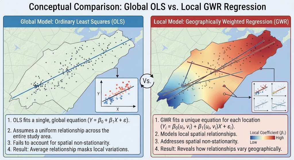
In traditional non-spatial statistics, Ordinary Least Squares (OLS) models a single global relationship across an entire study area. However, spatial data frequently exhibits spatial non-stationarity—a phenomenon where the strength and direction of relationships vary depending on geographic location. Geographically Weighted Regression (GWR) addresses this challenge by fitting localized regression equations at every sample point.
This tutorial explains the theoretical foundations of spatial regression, compares OLS and GWR, guides you through diagnosing model outputs, and provides a step-by-step workflow for ArcGIS Pro and QGIS.
1. Stationarity vs. Spatial Non-Stationarity in Spatial Modeling
Standard statistical models rely on the assumption of stationarity—the idea that the process being modeled operates identically everywhere in your study area.
+-------------------------------------------------------------------------+
|                          INPUT SPATIAL DATASETS                         |
|         Dependent Variable (Y) & Explanatory Variables (X1, X2...)       |
+------------------------------------+------------------------------------+
                                     |
             +-----------------------+-----------------------+
             |                                               |
             v                                               v
   +-------------------+                           +-------------------+
   |   GLOBAL MODEL    |                           |    LOCAL MODEL    |
   |  OLS Regression   |                           |   GWR Regression  |
   | Single Equation   |                           | Multiple Equations|
   +---------+---------+                           +---------+---------+
             |                                               |
             v                                               v
   Average Relationship                        Location-Specific
   Across Whole Study Area                     Coefficients & Local R²
Tobler’s First Law and Spatial Heterogeneity
Spatial datasets routinely break classical linear regression assumptions due to two primary spatial effects:
-
Spatial Autocorrelation: Nearby locations tend to have similar values (e.g., adjacent neighborhoods sharing similar median incomes).
-
Spatial Heterogeneity (Non-Stationarity): The structural relationship between variables changes over space. For instance, proximity to the coast might dramatically increase housing prices in a coastal city, but have little to no effect in a inland region.
When spatial non-stationarity is present, a global OLS model returns an average coefficient that may underpredict in some sub-regions and overpredict in others.
2. Ordinary Least Squares (OLS): Global Model Diagnostics
Before implementing local spatial models like GWR, you must build and evaluate a benchmark global OLS model.
The OLS Equation
The classic OLS linear model is defined as:
$$Y = \beta_0 + \beta_1 X_1 + \beta_2 X_2 + … + \beta_k X_k + \varepsilon$$
Where:
-
$Y$ is the dependent variable you are predicting.
-
$X_k$ are the independent explanatory variables.
-
$\beta_k$ are the calculated global regression coefficients (slopes).
-
$\varepsilon$ is the model error residual term.
Essential OLS Diagnostic Tests
When reviewing OLS geoprocessing reports in GIS, examine these critical diagnostic parameters:
| Diagnostic Statistic | Purpose / Interpretation | Target Threshold / Goal |
| R-Squared ($R^2$) / Adj. $R^2$ | Measures overall model goodness of fit (variance explained). | Higher values indicate better predictive power (0.0 to 1.0). |
| Joint F-Statistic / Wald Statistic | Tests overall statistical significance of the model model. | Low $p$-value ($p < 0.05$) indicates a statistically significant model. |
| Koenker (BP) Statistic | Tests for non-stationarity or heteroscedasticity. | If $p < 0.05$, relationships vary spatially—indicating a GWR model is appropriate. |
| Jarque-Bera Statistic | Evaluates whether model residuals are normally distributed. | If $p < 0.05$, residuals are non-normal, indicating omitted variable bias or non-linearity. |
| Variance Inflation Factor (VIF) | Checks for multicollinearity among explanatory variables. | VIF values should be $< 7.5$; values $> 10$ indicate redundant variables. |
3. Geographically Weighted Regression (GWR): Local Spatial Parameters
When the Koenker test in OLS reveals statistically significant non-stationarity, Geographically Weighted Regression (GWR) should be applied.
How GWR Works
Rather than computing a single global equation, GWR constructs a separate regression equation for every single observation point or polygon centroid in your dataset.
$$Y_i = \beta_0(u_i, v_i) + \sum_{k} \beta_k(u_i, v_i) X_{ik} + \varepsilon_i$$
Where $(u_i, v_i)$ represents the spatial X/Y geographic coordinates of the $i$-th sample point.
Observations closer to the target point $i$ exert greater weight in estimating local parameters than observations farther away, according to a spatial distance decay function (kernel).
Bandwidth Selection: Fixed vs. Adaptive
The bandwidth controls the spatial search radius or neighborhood size of the weighting kernel:
-
Fixed Bandwidth: Uses a constant distance radius across the entire study region. Ideal when sample points are evenly distributed in space.
-
Adaptive Bandwidth: Adjusts the search distance dynamically based on feature density. The kernel expands in sparse rural areas and contracts in dense urban centers to encompass a fixed number of nearest neighbors.
Pro Tip: Testing OLS Residuals for Spatial Autocorrelation
Never jump directly to GWR without first checking the spatial structure of your OLS residuals!
StdResid).
[Internal Link Context: Suggest linking to related article on Moran's I Spatial Autocorrelation].
4. Step-by-Step Tool Execution: Running OLS vs GWR Spatial Regression in GIS
Executing OLS and GWR in ArcGIS Pro
-
Run OLS Regression:
-
Open Geoprocessing Pane > Spatial Statistics Tools > Modeling Spatial Relationships > Ordinary Least Squares.
-
Set Input Feature Class, Unique ID Field, Dependent Variable, and Explanatory Variables.
-
Specify an Output Feature Class to output residual points.
-
Review the generated PDF / HTML diagnostic report summary table.
-
-
Run Geographically Weighted Regression:
-
Open Spatial Statistics Tools > Modeling Spatial Relationships > Geographically Weighted Regression (GWR).
-
Set Input Features, Dependent Variable, and Explanatory Variables.
-
Set Neighborhood Selection Method to Golden Search or AICc (Akaike Information Criterion) to determine the optimal bandwidth automatically.
-
Choose Neighborhood Type (Adaptive Conduct or Fixed Distance).
-
Click Run.
-
-
Map Local Coefficient Outputs:
-
Symbolize the GWR output feature layer using individual local coefficient fields ($\beta_{1\_var}$) to visualize how relationships change across regions.
-
Executing GWR in QGIS using Python / PySAL
While QGIS offers plugins such as GWmodel, Python integration through PySAL Spatial Analysis Libraries provides flexible script-based spatial modeling options within QGIS Python Console.
Python
import mgwr
from mgwr.gwr import GWR
from mgwr.sel_bw import Sel_BW

# Define coordinates, dependent, and independent variables
coords = list(zip(df['X'], df['Y']))
y = df['dependent_var'].values.reshape((-1, 1))
X = df[['var1', 'var2']].values

# Calculate optimal bandwidth using AICc
gwr_selector = Sel_BW(coords, y, X, kernel='bisquare', fixed=False)
gwr_bw = gwr_selector.search(criterion='AICc')

# Fit GWR model
gwr_model = GWR(coords, y, X, bandwidth=gwr_bw, kernel='bisquare')
gwr_results = gwr_model.fit()

print(f"Optimal Adaptive Bandwidth: {gwr_bw}")
print(f"Local R2 values: {gwr_results.R2}")
5. Frequently Asked Questions (FAQ)
When should I choose GWR over traditional OLS regression?
Use GWR when your OLS diagnostics show significant spatial non-stationarity (Koenker test $p < 0.05$) and spatial autocorrelation in the residuals (Global Moran’s I $p < 0.05$).
What does spatial non-stationarity mean in GIS?
Spatial non-stationarity means that the relationship between an independent variable and a dependent variable changes across geographic space, rather than remaining constant throughout the entire study area.
What is bandwidth selection in Geographically Weighted Regression?
Bandwidth defines the spatial neighborhood size around a target point used to weight nearby observations. It can be set to a fixed geographic distance or adapted dynamically based on point density.
6. Conclusion & Summary
Understanding the transition from global OLS to local GWR spatial regression is a essential milestone in advanced GIS and spatial statistics coursework. By diagnosing global model residuals, checking for spatial non-stationarity, and mapping local coefficients, you can account for spatial variations that traditional non-spatial models miss.
Key Takeaways:
-
Start with OLS to evaluate global relationships, multicollinearity (VIF), and residual distributions.
-
Test OLS residuals for spatial clustering using Global Moran’s I.
-
Apply GWR when non-stationarity is present, choosing appropriate bandwidth parameters to map localized spatial relationships.