
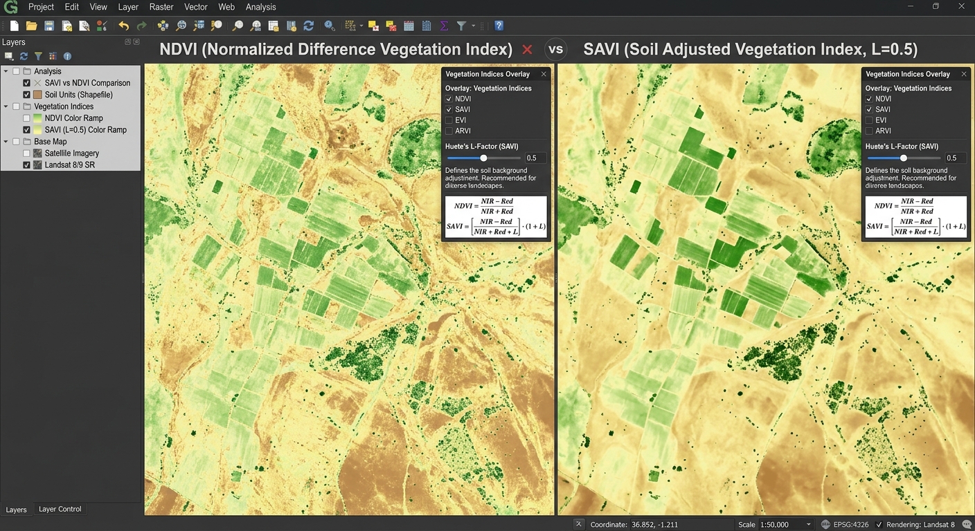
Soil Adjusted Vegetation Index SAVI vs NDVI GIS
1. Introduction: Why Compare SAVI and NDVI?
Vegetation indices are among the most widely used tools in agricultural remote sensing. They help researchers monitor crop growth, assess vegetation conditions, map rangelands, and investigate land degradation using satellite imagery.
The Normalized Difference Vegetation Index (NDVI) is a standard choice because it uses the contrast between near-infrared (NIR) and red reflectance to estimate vegetation greenness. However, NDVI has an important limitation: its values can be influenced by the brightness and spectral properties of the soil beneath sparse vegetation.
This becomes particularly important in arid and semi-arid environments, where vegetation does not completely cover the ground. A satellite pixel may contain a mixture of green plants, dry vegetation, and exposed soil. Consequently, the measured reflectance represents more than the plant canopy alone.
The Soil Adjusted Vegetation Index (SAVI) was developed by Huete in 1988 to reduce the influence of soil brightness on vegetation-index measurements. It introduces a soil adjustment factor, (L), to account for first-order soil–vegetation interactions. Huete (1988), A Soil-Adjusted Vegetation Index.
Both NDVI and SAVI are valuable in GIS, but the most appropriate choice depends on vegetation density, soil conditions, and the objective of the study.
2. The Problem with Soil Brightness in Remote Sensing
2.1 How NDVI Works
NDVI uses the difference between NIR and red reflectance, divided by their sum:
[
\boxed{NDVI=\frac{NIR-Red}{NIR+Red}}
]
Healthy green vegetation typically absorbs much of the incoming red radiation for photosynthesis while reflecting strongly in the NIR region because of its leaf structure.
This creates a contrast that makes NDVI useful for distinguishing greener vegetation from many non-vegetated surfaces.
NDVI generally produces values between −1 and +1 for nonnegative reflectance inputs with a nonzero denominator. Higher positive values often indicate greener or more abundant vegetation, while values near zero frequently occur over bare soil or sparsely vegetated surfaces. Interpretation depends on the land cover and environmental conditions. USGS NDVI overview.
2.2 Why Exposed Soil Affects NDVI
Imagine two agricultural fields with approximately the same sparse vegetation cover.
The first field has light-colored, dry sandy soil. The second has darker, moist soil. Even if the amount of vegetation is similar, their observed red and NIR reflectance may differ because the soil contributes to the signal recorded by the satellite.
This is known as soil background interference or soil background noise.
The problem occurs because the satellite measures the combined optical response of the vegetation and its background. When canopy cover is sparse, the soil contribution becomes proportionally more important.
As a result, NDVI may change because of differences in soil brightness or moisture, even when vegetation cover has not changed by the same amount.
This creates several challenges:
- Comparing crop vigor across fields with different soil types.
- Monitoring sparse vegetation in drylands and semi-arid regions.
- Estimating vegetation cover where exposed soil is common.
- Detecting changes in rangeland vegetation against varying soil backgrounds.
- Comparing agricultural plots with incomplete canopy cover.
NDVI does not completely remove these effects through normalization. The relationship between red and NIR soil reflectance can still influence the calculated index.
2.3 Why Soil Background Matters in Arid Vegetation Mapping
In deserts, savannas, dry grasslands, and semi-arid agricultural areas, a substantial proportion of each satellite pixel may consist of bare ground.
For example, a 30-metre Landsat pixel covers 900 square metres. If plants occupy only a small fraction of that area, the remaining soil contributes significantly to the measured reflectance.
NDVI can still provide useful information, but the soil contribution complicates its interpretation. SAVI addresses this problem by introducing an adjustment designed to reduce the first-order influence of the soil background.
3. Understanding SAVI: The Soil Adjusted Vegetation Index
3.1 The SAVI Formula
The Soil Adjusted Vegetation Index is calculated using the red and near-infrared bands, together with a soil adjustment factor.
[
\boxed{
SAVI=\frac{NIR-Red}{NIR+Red+L}\times(1+L)
}
]
Where:
- NIR: Near-infrared surface reflectance.
- Red: Red-band surface reflectance.
- (L): Soil adjustment factor.
- (1+L): Multiplicative adjustment that preserves the intended index scaling.
The key difference between SAVI and NDVI is the addition of (L) to the denominator and multiplication by (1+L).
This adjustment changes how the index responds to vegetation and soil reflectance. It is intended to reduce the influence of background brightness, particularly when vegetation cover is incomplete.
Important: Use reflectance values scaled to their physical decimal units, typically around 0–1, rather than unscaled integer digital numbers. The value of (L) must be compatible with the scale of the reflectance inputs.
3.2 What Is the Vegetation Index L Factor?
The vegetation index L factor controls the strength of the soil adjustment.
The original SAVI formulation allows (L) to vary with vegetation density and soil conditions. A value of (L=0.5) is commonly used as a practical default because it provides a useful compromise for many vegetation conditions.
A common starting guide is:
| Soil adjustment factor (L) | General vegetation condition | Practical interpretation |
|---|---|---|
| 1.0 | Very low vegetation cover | Stronger soil-background adjustment |
| 0.5 | Intermediate vegetation cover | Common default for mixed or partially covered land |
| 0.25 | Relatively high vegetation cover | Smaller soil-background adjustment |
| 0 | Any vegetation density | SAVI reduces mathematically to NDVI |
These are guidelines, not universal thresholds. The appropriate factor depends on the vegetation and soil characteristics in the study area. The USGS uses (L=0.5) for its standard Landsat SAVI product. USGS Landsat SAVI documentation.
3.3 Why Is L = 0.5 So Widely Used?
Setting (L=0.5) provides a practical balance for many land-cover conditions without requiring a separate adjustment for every pixel.
For this reason, it is frequently used in agricultural monitoring and regional vegetation mapping.
However, (L=0.5) does not automatically make SAVI the best index for every landscape. Sparse desert vegetation may benefit from a stronger adjustment, while dense vegetation may need less soil correction.
If you compare SAVI values across years or locations, keep the selected factor consistent unless you are deliberately investigating alternative parameter settings.
3.4 How SAVI Reduces Soil Background Influence
Consider the two fields described earlier, each containing sparse vegetation over a different soil background.
NDVI calculates its index directly from the red–NIR contrast and their sum. SAVI modifies that calculation by adding (L) to the denominator and applying the additional multiplier.
The resulting index is designed to reduce variation associated with soil brightness and emphasize the vegetation-related signal.
This does not eliminate every source of error. SAVI can still be affected by atmospheric conditions, sensor characteristics, shadows, vegetation structure, and differences in soil spectral properties.
It is therefore a soil-adjusted vegetation indicator, not a direct measurement of leaf area, biomass, or crop yield.
4. SAVI vs NDVI: Direct Comparison
The most important difference is not that one index is universally superior. It is that SAVI was designed to reduce a particular limitation of NDVI.
| Comparison criterion | NDVI | SAVI |
|---|---|---|
| Formula | ((NIR-Red)/(NIR+Red)) | (((NIR-Red)/(NIR+Red+L))(1+L)) |
| Main purpose | Estimate vegetation greenness and relative vegetation abundance | Estimate vegetation greenness while reducing soil background influence |
| Soil brightness sensitivity | More sensitive under sparse canopy conditions | Designed to reduce first-order soil brightness effects |
| Sparse vegetation | Useful, but soil effects can complicate interpretation | Often preferred when exposed soil is a major influence |
| Dense vegetation | Widely used, although it can saturate in dense canopies | Soil adjustment may be less important; use an appropriate lower (L) where justified |
| Arid and semi-arid regions | Useful for general monitoring | Particularly useful where vegetation cover is low and soil is exposed |
| Savannas and dry rangelands | Useful for seasonal greenness analysis | Helpful for reducing soil-background effects in open vegetation |
| Dense forests | Standard option for broad vegetation monitoring, with saturation limitations | Can be used, but soil adjustment may offer less benefit where canopy cover is nearly complete |
| Parameter selection | No soil adjustment parameter | Requires selection of (L) |
| Computational complexity | Simple two-band calculation | Simple two-band calculation with one additional parameter |
| Common applications | Crop monitoring, vegetation phenology, regional greenness mapping | Sparse vegetation mapping, dryland monitoring, and partially covered agricultural land |
Which Index Should You Choose?
Choose NDVI when your primary objective is routine vegetation monitoring, comparison with established NDVI time series, or broad-scale assessment in landscapes where soil background effects are less problematic.
Choose SAVI when exposed soil contributes strongly to the satellite signal, particularly in arid vegetation mapping, dry rangelands, and agricultural fields with incomplete canopy cover.
For very dense vegetation, neither index completely solves the limitations of spectral saturation. If the objective is to distinguish subtle differences in high-biomass forests, consider whether an index such as the Enhanced Vegetation Index (EVI) is more suitable.
5. Step-by-Step Calculation Guide in QGIS
The following workflow calculates NDVI and SAVI using satellite surface-reflectance imagery.
Step 1: Download and Prepare Satellite Imagery
You can use Landsat 8/9 or Sentinel-2 imagery.
| Satellite | Red band | NIR band | Native resolution |
|---|---|---|---|
| Landsat 8/9 | Band 4 | Band 5 | 30 m for both bands |
| Sentinel-2 | Band 4 | Band 8 | 10 m for both bands |
The band assignments are documented by the USGS for Landsat and in the Sentinel-2 technical specifications.
For reliable analysis, use atmospherically corrected surface-reflectance data, check cloud contamination, and ensure the selected bands represent the same area and pixel grid.
Step 2: Load the Bands into QGIS
Open QGIS and import your red and NIR rasters.
- Select Layer → Add Layer → Add Raster Layer.
- Browse to your downloaded satellite imagery.
- Load the red and NIR bands.
- Check their coordinate reference systems, extents, and resolutions.
- Mask clouds, shadows, and invalid pixels where necessary.
For a Landsat time series, Collection 2 Level-2 Surface Reflectance products are useful. Their stored digital numbers require scaling and an additive offset before applying SAVI.
The USGS scaling equation is:
[
SR=(DN\times0.0000275)-0.2
]
where (DN) is the stored digital number and (SR) is the surface-reflectance value. USGS scaling instructions.
Prepare both the Red and NIR layers as reflectance values before proceeding. For Sentinel-2, check the product metadata for the appropriate reflectance quantification and any applicable offsets.
Step 3: Calculate NDVI
Open Raster → Raster Calculator in QGIS.
Assume your prepared layers are named NIR_SR and RED_SR. Enter the following expression:
("NIR_SR@1" - "RED_SR@1") /
("NIR_SR@1" + "RED_SR@1")
Choose an output filename such as:
NDVI.tif
Click OK or Run, depending on the calculator interface.
The output contains a calculated NDVI value for each valid pixel.
Step 4: Calculate SAVI
Open Raster Calculator again.
For the standard (L=0.5) setting, enter:
(("NIR_SR@1" - "RED_SR@1") /
("NIR_SR@1" + "RED_SR@1" + 0.5)) * 1.5
Save the output as:
SAVI_L05.tif
The expression implements:
[
SAVI=\frac{NIR-Red}{NIR+Red+0.5}\times1.5
]
Check the layer names carefully. In QGIS, raster bands are referenced using the layer name followed by @ and the band number. The names in your project may differ from the examples above. The QGIS Raster Calculator documentation explains raster expressions and output settings.
Step 5: Apply Symbology
Right-click each output raster and select Properties → Symbology.
Choose a single-band pseudocolor renderer and apply a sequential color ramp.
For example, use lighter shades for lower index values and darker green shades for higher values. Keep the same color logic when comparing the two indices.
Interpretation should account for the study area:
- Low or negative values may indicate bare surfaces, water, or non-green vegetation.
- Moderate positive values often occur in grasslands, sparse vegetation, or growing crops.
- Higher positive values commonly indicate greener vegetation or denser canopies.
These are general guides, not universal classification thresholds. Use reference imagery or field observations when assigning specific land-cover meanings.
Step 6: Compare SAVI with NDVI
Load both index rasters side by side or create a map layout with two synchronized map panels.
Inspect locations where soil is strongly exposed and compare how each index represents them.
For a quantitative comparison, calculate raster statistics or sample the index values at locations representing sparse vegetation, bare soil, and dense vegetation.
A difference raster can also be calculated:
"SAVI_L05@1" - "NDVI@1"Save it as SAVI_minus_NDVI.tif.
This difference reveals how the two index calculations vary spatially. It does not directly measure the amount of soil correction or establish which index is more accurate. That judgment requires suitable reference data.
6. Calculating SAVI in ArcGIS Pro
The same approach can be implemented in ArcGIS Pro using the Raster Calculator, provided you have access to the Spatial Analyst or Image Analyst extension.
Step 1: Add the Red and NIR Layers
Load the red and NIR surface-reflectance bands into your project and confirm their alignment.
Step 2: Open Raster Calculator
In the Geoprocessing pane, search for Raster Calculator under Spatial Analyst Tools.
Step 3: Enter the SAVI Expression
Assuming your reflectance layers are named NIR_SR and RED_SR, use:
(
    (Float("NIR_SR") - Float("RED_SR")) /
    (Float("NIR_SR") + Float("RED_SR") + 0.5)
) * 1.5
Specify an output raster such as SAVI_L05.tif and run the tool.
The Float() function ensures floating-point calculations are used. Set the appropriate output coordinate system, cell size, extent, and snap raster so the result aligns with the source bands.
Official documentation: ArcGIS Pro Raster Calculator.
7. Practical Recommendations for Agricultural Remote Sensing
The SAVI-versus-NDVI decision should be based on the vegetation conditions and research objective.
For arid and semi-arid vegetation mapping, SAVI with (L=0.5) is a reasonable initial choice when exposed soil is substantial. Compare (L=0.25), (0.5), and (1.0) where vegetation density varies considerably, and document the selected value.
For crop monitoring, consider the crop growth stage. Early-season crops often leave more soil exposed, making soil adjustment useful. Later in the season, as the canopy closes, the benefit may become smaller.
For long-term vegetation change detection, maintain consistent band selection, reflectance processing, cloud masking, and SAVI parameters across dates. If different sensors are used, evaluate their spectral and spatial differences before interpreting changes.
For dense forests, NDVI remains a practical baseline, but saturation and canopy complexity should be considered. SAVI should not be assumed to solve those problems simply because it includes a soil-adjustment term.
Most importantly, neither index directly measures crop yield, soil moisture, biomass, or fractional vegetation cover without additional modeling and validation.
8. Summary and Key Takeaways
The comparison of SAVI vs NDVI in GIS illustrates why selecting an appropriate vegetation index matters in agricultural remote sensing.
NDVI is a widely used measure of vegetation greenness and relative abundance, but soil brightness can affect its results when vegetation cover is sparse.
SAVI modifies the NDVI equation by adding the soil adjustment factor (L) and multiplying by (1+L). A value of (L=0.5) is a common default for intermediate vegetation density, while other values may be appropriate depending on canopy cover and soil conditions.
For practical GIS work, prepare reflectance data correctly, calculate both indices when useful, and interpret their spatial differences in the context of the landscape.
The key lesson: NDVI is an excellent general-purpose vegetation index, while SAVI is particularly valuable when exposed soil contributes substantially to the signal. Choosing between them should reflect the actual vegetation and soil conditions rather than a universal preference for one formula.
References
- Huete, A. R. (1988). A soil-adjusted vegetation index (SAVI). Remote Sensing of Environment, 25(3), 295–309.
- USGS: Landsat Soil Adjusted Vegetation Index.
- USGS: NDVI and remote sensing phenology.
- QGIS: Raster analysis and Raster Calculator.