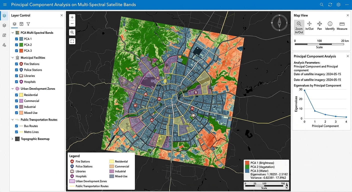
Principal Component Analysis (PCA) on Multi-Spectral Satellite Bands for Dimensionality Reduction

 

1. Introduction: Why Apply PCA to Satellite Imagery?

Applying Principal Component Analysis on Multi-Spectral Satellite Bands is a vital technique for reducing dimensionality in remote sensing workflows. Modern Earth observation satellites capture information about the same landscape across multiple spectral bands. Landsat and Sentinel-2, for example, record reflected energy in visible, near-infrared, and shortwave-infrared wavelengths. These bands reveal different characteristics of vegetation, soil, water, and built-up surfaces.

However, many spectral bands contain overlapping information. Vegetated areas may produce similar spatial patterns in several visible and infrared bands, while other bands respond to related surface properties.

This overlap is known as spectral redundancy and is often associated with multicollinearity among spectral variables.

When a remote sensing analyst uses many correlated bands as inputs to a classification or regression model, the workflow can require additional memory, storage, and computation. Some statistical algorithms may also become harder to interpret when their predictors are strongly correlated.

Principal Component Analysis (PCA) addresses this problem by transforming the original spectral bands into a new set of uncorrelated variables called principal components. These components are ordered according to how much variance they explain in the input data.

Rather than analyzing every original band, an analyst may be able to use only the leading components while retaining most of the overall variation.

For example, a land-cover classification might use ten original spectral bands. If the first four principal components capture most of the relevant spectral variation, using those four components could reduce the input dimensionality of the classification workflow.

However, retaining fewer components always involves a trade-off: some information is discarded, and low-variance components can still contain valuable information for distinguishing particular land-cover classes.

This tutorial explains how PCA works, how to interpret its outputs, and how to perform PCA raster processing in QGIS and ArcGIS Pro.

2. Understanding Spectral Redundancy and Multicollinearity

2.1 Why Are Satellite Bands Correlated?

Consider a Landsat image containing several spectral bands. Many areas covered by healthy vegetation will produce characteristic reflectance patterns across the visible and infrared regions. Some of these bands may consequently show similar spatial variation.

For instance:

• Vegetation absorbs much of the incoming red radiation and reflects strongly in the near-infrared region.
• Water often absorbs strongly in the near-infrared and shortwave-infrared regions.
• Bare soil reflectance may vary across several bands according to its mineral composition, moisture, and surface properties.
• Urban materials may produce related spectral responses across multiple bands.

Because the same surface affects several bands, the resulting measurements are not necessarily independent.

In statistical analysis, strong relationships between predictor variables are commonly associated with multicollinearity.

2.2 Why Redundant Bands Can Be a Problem

Suppose you are mapping land cover using ten spectral bands.

Your dataset may contain considerable repeated information about the same dominant landscape patterns. Processing every band may increase the cost of storing, moving, and analyzing the data.

Dimensionality reduction can help by replacing the original variables with a smaller number of components.

Potential advantages include:

• Reduced dimensionality: Fewer input variables for subsequent analysis.
• Band decorrelation: Linear correlations between the resulting principal components are removed.
• Computational efficiency: Some classification and regression workflows become faster when fewer features are processed.
• Visualization: A small set of components can reveal spectral contrasts not obvious in the original bands.
• Exploratory analysis: Lower-variance components may reveal subtle spectral differences or unusual observations.

PCA does not automatically remove noise or improve classification accuracy. Its primary objective is to maximize explained variance, not to distinguish genuine environmental information from noise.

The main benefit is that redundant spectral information can often be represented more compactly.

3. How Principal Component Analysis Works on Satellite Imagery

PCA transforms a group of correlated input bands into a new set of orthogonal linear combinations.

These transformed variables are called Principal Component 1 (PC1), Principal Component 2 (PC2), Principal Component 3 (PC3), and so on.

3.1 The Basic PCA Principle

Imagine a multiband satellite image containing six spectral bands.

Each valid pixel has six associated reflectance values. PCA treats these measurements as a six-dimensional observation and identifies new directions through the data that capture its variance.

The first direction captures the greatest possible variance. The second captures the greatest remaining variance while being orthogonal to the first. The process continues for the remaining components.

Conceptually, the transformation follows this sequence:

ORIGINAL SATELLITE BANDS
B1  B2  B3  B4  B5  B6
         |
         v
  PCA TRANSFORMATION
  (eigenvectors and eigenvalues)
         |
         v
PRINCIPAL COMPONENTS
PC1  PC2  PC3  PC4  PC5  PC6
         |
         v
SELECT LEADING COMPONENTS
        PC1 PC2 PC3
         |
         v
LAND-COVER CLASSIFICATION

The output components are arranged in descending order of explained variance.

If six components are calculated from six input bands, the full transformation retains the original information, apart from numerical precision and any changes caused by preprocessing or output rescaling. The dimensionality reduction occurs when only a subset of components is retained.

3.2 The Mathematical Foundation

Let the input satellite bands form a data matrix (X), where each row represents a valid pixel and each column represents a spectral band.

The data are centered by subtracting the mean of each input band. PCA then finds eigenvectors of the selected covariance or correlation matrix.

A principal component can be expressed as:

[
PC_k=\sum_{j=1}^{p}a_{jk}(B_j-\bar{B}_j)
]

Where:

• (PC_k) is the score of component (k) for a pixel.
• (p) is the number of input bands.
• (B_j) is the reflectance value in input band (j).
• (\bar{B}_j) is the mean value of that band.
• (a_{jk}) is the loading or coefficient associated with band (j) in component (k).

The coefficients determine how much each original band contributes to the component.

For example, if visible, near-infrared, and shortwave-infrared bands have large coefficients in PC1 with similar signs, the component may represent broad brightness variation. If some bands have positive coefficients and others have negative coefficients, the component may emphasize a spectral contrast.

The exact meaning depends on the calculated coefficients, not simply on the component’s number.

3.3 Eigenvalues and Explained Variance

An eigenvalue measures how much variance is associated with a principal component.

The percentage of variance explained by component (k) is:

[
P_k=\frac{\lambda_k}{\sum_{j=1}^{p}\lambda_j}\times100
]

Where:

• (\lambda_k) is the eigenvalue for component (k).
• The denominator is the sum of all component eigenvalues.

Cumulative explained variance is the running total of the percentages:

[
C_m=\sum_{k=1}^{m}P_k
]

This tells you how much of the original total variance is represented by the first (m) components.

For example, if PC1 explains 65% of the variance and PC2 explains another 20%, the first two components together explain 85%.

That figure can help guide component selection, although it does not prove that 85% of the information relevant to a particular classification task has been retained.

3.4 Covariance PCA Versus Correlation PCA

An important preprocessing decision is whether PCA should use the covariance matrix or the correlation matrix.

Covariance-based PCA uses centered inputs without scaling each band to unit variance. For consistently scaled surface-reflectance bands, this is a common starting point because all bands share the same physical units.

Correlation-based PCA standardizes each band to have unit variance before calculating the transformation. This gives bands comparable variance in the PCA calculation.

Standardization can be useful when input variables have substantially different scales or units. However, it can also give relatively noisy or low-variance bands more influence than they would receive in covariance-based PCA.

For multispectral imagery, select the approach based on the nature of the inputs and document the choice. Do not assume that normalization is always necessary, or that unscaled integer digital numbers are suitable inputs.

4. Interpreting the Principal Components

A major advantage of PCA is that it can expose different patterns of spectral variation in separate raster layers.

However, PC1 does not always represent brightness, PC2 does not always separate vegetation from soil, and PC3 does not always represent noise. These are common possibilities, not universal rules.

The actual interpretation must be based on the eigenvectors or loadings, variance statistics, and spatial appearance of the components.

4.1 PC1: Dominant Spectral Variation

PC1 captures the greatest variance among the input bands.

In multispectral imagery, many bands respond to overall scene brightness and broad surface differences. Consequently, PC1 often resembles an overall brightness or albedo-related image, especially when the input bands are positively correlated.

Typical visual patterns may include:

• Broad differences between bright and dark surfaces.
• Strong contrast between some land-cover types.
• Large-scale spatial variation shared by multiple spectral bands.

However, PC1 represents the direction of maximum statistical variance, not a pure measurement of surface brightness or albedo.

Atmospheric effects, illumination differences, and other sources of variation can influence it.

4.2 PC2: Secondary Spectral Contrasts

PC2 captures the greatest remaining variance after the first component.

Because it is orthogonal to PC1, it can emphasize relationships among bands that are different from the dominant variation.

Depending on the input bands and landscape, PC2 may reveal contrasts associated with:

• Vegetation and soil.
• Moisture differences.
• Differences between visible and infrared reflectance.
• Built-up materials and other land-cover types.

To interpret PC2, inspect the signs and magnitudes of its loadings. Large coefficients of opposite sign for vegetation-sensitive and soil-sensitive bands may suggest a spectral contrast between these surfaces.

The interpretation should still be tested against the actual imagery and known land-cover locations.

4.3 PC3 and Later Components: Subtle Variation

Later components account for progressively smaller proportions of the total variance.

These components may reveal:

• Localized geological or mineralogical contrasts.
• Subtle vegetation differences.
• Boundaries between land-cover classes.
• Rare or spatially localized features.
• Sensor noise, atmospheric artefacts, or other unwanted variation.

Low variance does not necessarily mean that a component is useless. A component explaining only a small fraction of total variance could still distinguish a rare but important land-cover class.

Likewise, a component with high variance could mainly represent illumination or atmospheric differences rather than useful classification information.

Therefore, inspect the components instead of automatically discarding everything after PC3.

5. Step-by-Step PCA Workflow in QGIS

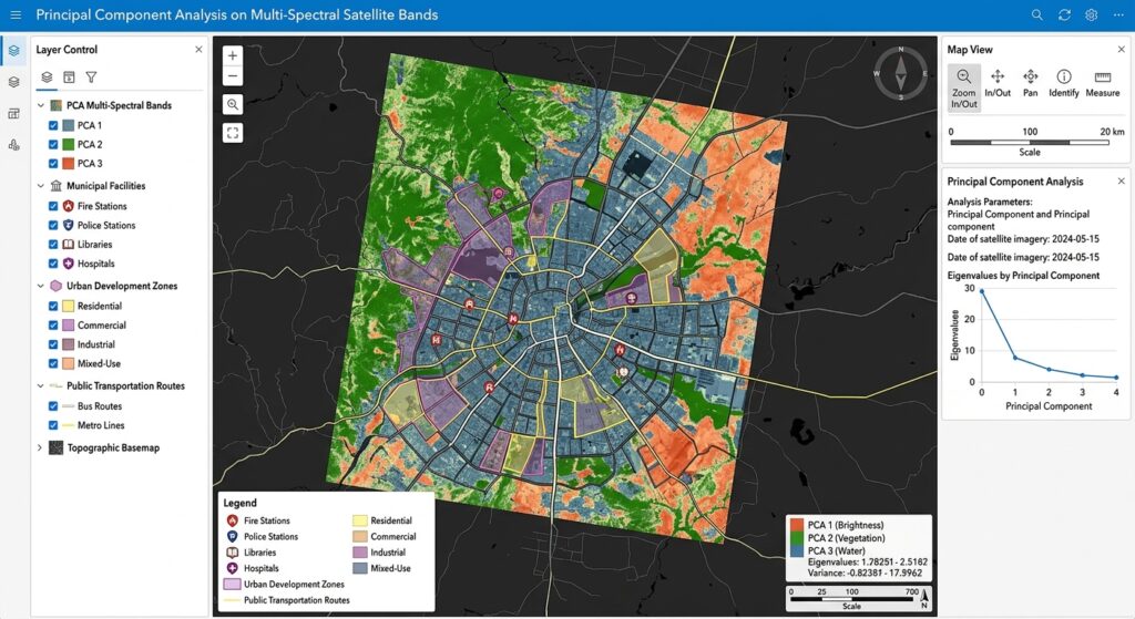
QGIS can prepare the input raster stack and run PCA through its integrated GRASS GIS processing tools. The GRASS i.pca module calculates principal components from multiple raster inputs and stores information about eigenvalues and eigenvectors in raster history metadata.

Official reference: GRASS GIS i.pca documentation.

Step 1: Download and Prepare the Satellite Bands

Select a multispectral scene from a suitable source, such as Landsat or Sentinel-2.

For a Landsat 8/9 land-cover study, you might use the following bands:

Band	Spectral region	Potential information
Band 2	Blue	Water, atmospheric effects, surface reflectance
Band 3	Green	Vegetation and visible surface properties
Band 4	Red	Vegetation absorption and land-cover differences
Band 5	Near-infrared	Vegetation structure and biomass-related variation
Band 6	SWIR 1	Moisture and surface-material variation
Band 7	SWIR 2	Moisture and mineral-related spectral differences

For this example, six bands provide a manageable starting dataset.

Before PCA:

1. Prefer atmospherically corrected surface-reflectance products for land-cover analysis.
2. Apply the correct reflectance scale factors and offsets where required.
3. Mask clouds, cloud shadows, and invalid pixels.
4. Confirm that each selected band covers the same study area.
5. Ensure that all bands share a consistent pixel grid and spatial resolution.
6. Exclude quality-assurance masks and unrelated non-spectral layers from the PCA input.

PCA can be strongly affected by poor preprocessing. Cloud contamination, inconsistent extents, and large areas of NoData can distort the statistics.

Step 2: Build a Virtual Raster Stack

A virtual raster (VRT) lets you organize several single-band rasters into one multiband dataset without immediately creating a large physical copy of the data.

In QGIS:

1. Open Processing Toolbox.
2. Search for Build Virtual Raster.
3. Add the selected spectral bands in a consistent order.
4. Enable Place each input file into a separate band.
5. Select the appropriate resolution and output extent.
6. Save the output as multispectral_stack.vrt.

The separate-band option is important. Without it, the tool may mosaic inputs rather than stack them into individual bands.

See the QGIS Build Virtual Raster documentation.

A VRT is a virtual reference to its source files, not an independent copy of them. Keep the source files accessible, and use a persistent physical raster stack when the next application or analysis requires one.

Practical note: The GRASS i.pca module accepts multiple raster layers as separate inputs. You can use the organized stack to check the imagery, but when running i.pca, select the individual single-band layers as the input list.

Step 3: Open the GRASS PCA Tool

In QGIS, open the Processing Toolbox and search for:

i.pca

Look for the GRASS GIS Principal components analysis (PCA) for image processing tool.

If the tool is not available, verify that the GRASS provider is enabled in QGIS Processing settings and that the GRASS installation is correctly configured.

Set the input rasters to your prepared spectral bands, for example:

• Blue
• Green
• Red
• NIR
• SWIR 1
• SWIR 2

Specify an output basename such as:

landsat_pca

The tool will produce component rasters with numerical suffixes such as landsat_pca.1, landsat_pca.2, and so on.

By default, GRASS may rescale the outputs to an 8-bit range of 0–255 for display. For floating-point component scores, set the rescaling range to 0,0, which instructs the tool not to rescale the results.

Run the process and inspect the generated layers.

Step 4: Inspect PC1, PC2, and PC3

Load the output component rasters into QGIS and examine them individually.

For each raster:

1. Open Layer Properties → Symbology.
2. Select a single-band grayscale or pseudocolor renderer.
3. Stretch the display to the actual data range.
4. Compare the output with a true-colour or false-colour satellite composite.
5. Identify whether visible patterns correspond to known surface types.

A default grayscale stretch may initially make a component look almost entirely black or white. This is often a display-range issue rather than a calculation error.

Remember that the signs of PCA eigenvectors are mathematically arbitrary. A component and its sign-reversed equivalent represent the same statistical direction, so a reversed brightness pattern does not automatically indicate an incorrect PCA result.

Step 5: Inspect Eigenvalues and Explained Variance

The component images show the spatial pattern, but they do not tell you how much variance each component explains.

The GRASS i.pca module stores eigenvalue, eigenvector, and percentage-importance information in its output raster history.

To inspect this information in a GRASS environment, use the r.info command with the history flag:

r.info -h landsat_pca.1

Review the output for the component eigenvalues, loadings, and explained variance percentages.

For a clearer summary, organize the results into a table:

Component	Eigenvalue	Variance explained	Cumulative variance
PC1	Example only	65%	65%
PC2	Example only	20%	85%
PC3	Example only	9%	94%
PC4	Example only	4%	98%
PC5	Example only	1.5%	99.5%
PC6	Example only	0.5%	100%

These percentages are illustrative, not measured results from your imagery.

To calculate the cumulative percentage, add the explained variance sequentially. In the example, the first three components explain 94% of the total variance.

For projects requiring a clean CSV table and explicit output files for loadings and eigenvalues, ArcGIS Pro’s Principal Components tool also provides an output data file containing these statistics.

Step 6: Choose Components for Classification

Suppose your analysis produces six components, and the variance table shows that the first three account for 94% of total variance.

You could begin by testing PC1, PC2, and PC3 as input features for a land-cover classification.

Compare the resulting classification against a model using the original six spectral bands.

Evaluate:

• Overall classification accuracy.
• Class-specific producer’s and user’s accuracy.
• Confusion between similar land-cover categories.
• Performance for uncommon classes.
• Computational time and memory requirements.

A high cumulative variance percentage provides a useful starting point, but it does not guarantee equal classification accuracy.

When subtle differences between land-cover classes are important, retaining additional components may improve the result even if those components explain comparatively little total variance.

6. Step-by-Step PCA Workflow in ArcGIS Pro

ArcGIS Pro offers a dedicated Principal Components tool in the Spatial Analyst toolbox. It generates a multiband principal-component raster and can provide a text or tabular output containing the PCA statistics.

Official reference: ArcGIS Pro Principal Components.

Step 1: Prepare and Stack the Bands

Load the required satellite bands into your ArcGIS Pro project.

Use Composite Bands to create a single multiband raster from the selected spectral inputs, if necessary.

Ensure that the bands share a suitable common extent, grid, resolution, and projection. Apply the same cloud masking and reflectance preparation used in the QGIS workflow.

Step 2: Open the Principal Components Tool

Open the Geoprocessing pane and search for:

Principal Components

The tool is available under Spatial Analyst Tools → Multivariate and requires the Spatial Analyst extension.

Step 3: Configure the Analysis

Specify:

• Input Raster Bands: The selected spectral bands or multiband raster.
• Number of Principal Components: The number of components to generate, up to the number of input bands.
• Output Data File: A file for the PCA statistics, such as pca_statistics.csv or pca_statistics.txt, where supported by the chosen output format.

For an initial analysis, generating all components is useful because it lets you inspect their variance distribution before deciding which ones to retain.

Run the tool to generate the multiband PCA output.

Step 4: Review the Statistics

Open the output data file and inspect:

• Correlation and covariance matrices.
• Eigenvalues and eigenvectors.
• Percentage of variance explained by each component.
• Cumulative explained variance.

The eigenvalues show how variance is distributed among the components, while the eigenvectors or loadings describe how the original bands contribute to each component.

Use these outputs alongside the component images to understand the spectral information captured in each layer.

Step 5: Export the Selected Components

If the first three components are sufficient for your classification experiment, extract PC1, PC2, and PC3 from the multiband output using an appropriate band-extraction workflow.

Save the selected components as persistent rasters and use them as input features in your classification model.

For large regional workflows, consider a consistent raster format, appropriate compression, and a defined analysis grid to avoid unnecessary data conversion.

7. Practical Interpretation: What the Variance Table Tells You

The variance table helps determine whether PCA has successfully compressed the input data into a smaller set of components.

Consider two hypothetical datasets.

Dataset A: PC1 explains 75% of the variance, PC2 explains 15%, and PC3 explains 7%. The first three components explain 97% of total variance. This suggests that a small subset captures most of the overall variation.

Dataset B: Variance is distributed more evenly across six components. In that case, selecting only the first two or three components would discard a more substantial share of the original variance.

These examples illustrate why the variance table matters. The number of components to retain should be based on both the variance distribution and the purpose of the analysis.

Avoid Choosing Components by Variance Alone

The highest-variance components are not necessarily the most useful for every task.

For example, a rare mineral signature or a small land-cover class may account for little of the total scene variance but remain essential to the research question.

If your goal is geological mapping, crop discrimination, or a rare-class detection task, evaluate whether later components contain relevant spectral information before discarding them.

PCA is an unsupervised linear transformation. It does not use the classification labels to identify which features best separate your target classes.

8. Common Mistakes to Avoid

• Using inconsistent band grids: Misaligned raster cells can compromise the pixel-by-pixel multivariate analysis.
• Mixing incompatible data scales: Unscaled digital numbers or input bands with incomparable units can distort the covariance structure.
• Including cloud-contaminated pixels: Clouds and shadows may dominate some components and obscure land-cover variation.
• Interpreting PC1 and PC2 as fixed physical variables: Their meaning depends on the data, preprocessing, and calculated loadings.
• Discarding all low-variance components: A component with little overall variance can still be important for distinguishing a specific class.
• Assuming PCA removes all noise: PCA prioritizes total variance, which may include noise and unwanted environmental variation.
• Comparing components from independently fitted PCAs without alignment: Component signs and directions can change when the input data or preprocessing changes.
• Reporting explained variance as classification accuracy: Variance retention and predictive performance are different measures and must be evaluated separately.

9. Conclusion

Principal Component Analysis is a useful technique for reducing spectral dimensionality in multispectral satellite imagery. It transforms correlated input bands into orthogonal components ordered according to explained variance, providing a compact representation of major spectral patterns.

In QGIS, PCA can be performed using the GRASS i.pca tool, while ArcGIS Pro provides a dedicated Principal Components geoprocessing tool with outputs for the component raster and associated statistics.

For a defensible workflow, prepare the imagery consistently, examine component loadings and eigenvalues, interpret the component rasters visually, and test the selected components in the intended classification or analytical task.

The central lesson: PCA identifies the directions of greatest variation in satellite data. The analyst must determine which of those directions are meaningful for the specific remote sensing problem.

References

• GRASS GIS: i.pca documentation — PCA inputs, output components, normalization, and eigenvalue history.
• QGIS: Build Virtual Raster — preparing multiband raster stacks.
• ArcGIS Pro: Principal Components — PCA tool parameters, output statistics, and variance calculation.
• ArcGIS Pro: Reduce Spectral Bands — PCA versus Minimum Noise Fraction for spectral dimensionality reduction.