Calculating Built-Up Index (NDBI) in QGIS for Urban Expansion Analysis

 

1. Introduction: What Is the Normalized Difference Built-Up Index?

Calculating Built-Up Index in QGIS is an essential remote sensing technique for monitoring urban expansion and impervious surfaces over time. Rapid urbanization transforms natural landscapes into buildings, roads, parking areas, and other impervious surfaces. Monitoring these changes is important for urban planning, infrastructure development, environmental management, and agricultural land conservation.

Satellite remote sensing makes it possible to investigate urban expansion across large geographical areas without surveying every building on the ground.

One commonly used technique is the Normalized Difference Built-Up Index (NDBI). This spectral index uses differences in how the Earth’s surface reflects shortwave infrared and near-infrared radiation to highlight areas that may contain built-up surfaces.

NDBI is particularly useful in urban land use mapping, where analysts need to identify candidate built-up areas and investigate how they change over time.

1.1 The NDBI Formula

The Normalized Difference Built-Up Index is calculated using the following equation:

[
\boxed{\mathrm{NDBI}=\frac{SWIR-NIR}{SWIR+NIR}}
]

Where:

• SWIR (Shortwave Infrared): Measures reflected energy in the shortwave infrared region.
• NIR (Near-Infrared): Measures reflected energy in the near-infrared region.

The index typically produces values between -1 and +1 when valid nonnegative reflectance values are used and the denominator is nonzero.

Common interpretations include:

NDBI value	General interpretation
Negative values	Often associated with vegetation or water, depending on the surface
Values near zero	May represent mixed surfaces or other land-cover types
Positive values	May indicate built-up surfaces or exposed bare soil

Important: Positive NDBI values do not automatically mean that a pixel contains a building or a concrete surface. Bare soil, dry agricultural fields, construction sites, and other exposed ground can also produce positive values. The index is best used as an indicator of potential built-up areas rather than a definitive land-cover classifier. Research on NDBI limitations.

1.2 Why Use NDBI for Urban Expansion Analysis?

NDBI helps researchers investigate the spatial distribution of potential built-up surfaces and how those patterns change between satellite acquisition dates.

Typical applications include:

• Mapping the expansion of residential and commercial development.
• Identifying potential conversion of agricultural land into developed land.
• Comparing urban growth between two or more years.
• Supporting studies of impervious surfaces and urban heat islands.
• Identifying rapidly developing peri-urban areas.

In this tutorial, you will calculate NDBI in QGIS, remove water pixels from the analysis, create a preliminary built-up classification, and compare two dates to investigate urban expansion.

2. Data Requirements: Landsat 8/9 or Sentinel-2

Before opening QGIS, obtain suitable satellite imagery covering your study area.

Two widely used data sources are Landsat and Sentinel-2.

2.1 Landsat 8 and Landsat 9

Landsat provides multispectral imagery with a 30-metre spatial resolution for the optical bands used in this workflow.

For Landsat 8/9 Operational Land Imager imagery, use the following bands:

Band	Spectral region	Application	Spatial resolution
Band 3	Green	NDWI water detection	30 m
Band 4	Red	Optional NDVI vegetation filtering	30 m
Band 5	Near-Infrared (NIR)	NDBI and NDWI	30 m
Band 6	Shortwave Infrared 1 (SWIR1)	NDBI	30 m

The official USGS Landsat band reference confirms these band assignments.

For a reproducible urban expansion study, consider downloading Landsat Collection 2 Level-2 Surface Reflectance imagery. Surface reflectance products are atmospherically corrected and more appropriate for comparing dates than uncorrected raw imagery.

Download imagery through USGS EarthExplorer.

For a 2015-versus-2025 comparison, Landsat 8 imagery can provide a consistent sensor across both dates. Select scenes with low cloud cover and similar seasonal conditions.

2.2 Sentinel-2 Imagery

Sentinel-2 provides multispectral imagery with different spatial resolutions depending on the band.

Band	Spectral region	Application	Spatial resolution
B3	Green	NDWI	10 m
B4	Red	Optional NDVI	10 m
B8	Near-Infrared (NIR)	NDBI and NDWI	10 m
B11	Shortwave Infrared 1	NDBI	20 m

Sentinel-2 B11 has a native 20-metre resolution, while B8 has a 10-metre resolution. To calculate NDBI correctly, the bands must be aligned to a common grid and resolution. A 20-metre analysis grid is a sensible option because it preserves the native resolution of B11. Resampling B11 to 10 metres does not create additional spatial detail. Copernicus Sentinel-2 band specifications.

Download Sentinel-2 Level-2A Surface Reflectance imagery from the Copernicus Browser.

2.3 Essential Preparation Before Analysis

Regardless of your chosen satellite, check that:

• The imagery covers the same study area and has a suitable coordinate reference system.
• Clouds, cloud shadows, and invalid pixels have been masked.
• The selected dates represent comparable seasons where possible.
• The input bands have compatible dimensions, pixel alignment, and spatial extent.
• Reflectance scaling and offsets have been handled correctly.

The final point is particularly important for Landsat Collection 2 Level-2 products. Their surface-reflectance digital numbers must be converted using the scale factor and additive offset provided by USGS.

For Landsat Collection 2 Surface Reflectance:

[
SR=(DN\times0.0000275)-0.2
]

Where (DN) is the stored digital number and (SR) is the surface reflectance. Applying the scale factor without the offset can distort NDBI values because the offset does not cancel out in the normalized-difference equation. See the USGS scaling instructions.

3. Step-by-Step Workflow: Calculating NDBI in QGIS

The following instructions use the QGIS Processing Toolbox Raster Calculator. The same principles apply to Sentinel-2 imagery after aligning its input bands.

Step 1: Download and Import the Satellite Bands

First, download your satellite scene and extract its files.

For a Landsat 8/9 Level-2 product, locate the files corresponding to:

• SR_B3.TIF — Green
• SR_B4.TIF — Red
• SR_B5.TIF — NIR
• SR_B6.TIF — SWIR1
• QA_PIXEL.TIF — Pixel quality information for cloud and shadow masking

The exact filenames may contain additional product identifiers.

Open QGIS and load the relevant rasters:

1. Start a new QGIS project.
2. Select Layer → Add Layer → Add Raster Layer.
3. Browse to the extracted satellite files.
4. Load the required bands.
5. Inspect their CRS, extent, dimensions, and pixel resolution.
6. Mask clouds, shadows, and invalid pixels before calculating the index.

You can inspect a natural-colour view using Red, Green, and Blue composites where the required bands are available. For Landsat 8/9, a natural-colour composite commonly uses Bands 4, 3, and 2.

This visual inspection helps you identify cloud contamination, scene boundaries, and obvious differences in the study area.

Screenshot cue: Show the QGIS Layers panel containing the imported Landsat bands and the satellite image displayed on the map canvas.

Step 2: Apply Reflectance Scaling to Landsat Bands

If you are using Landsat Collection 2 Level-2 Surface Reflectance data, convert the relevant bands to reflectance before calculating NDBI.

Open Processing Toolbox → Raster analysis → Raster calculator.

For the SWIR1 band, use the following expression, replacing the layer reference with the exact name in your QGIS project:

"SR_B6@1" * 0.0000275 - 0.2

Save the output as:

SWIR1_SR.tif

Repeat the process for the NIR band:

"SR_B5@1" * 0.0000275 - 0.2

Save the output as:

NIR_SR.tif

Use the same scaling convention for the Green and Red bands if you will calculate NDWI or NDVI from Landsat Collection 2 data.

The layer references above are examples. Select the correct names from the Raster Calculator’s available input layers.

If your imagery is already stored as properly scaled reflectance values, do not apply the scaling a second time. For Sentinel-2, check the product metadata and processing baseline for the applicable scale and offset rather than assuming that every downloaded product uses the same convention.

Step 3: Calculate NDBI Using the Raster Calculator

You now have the two input reflectance layers required for NDBI.

Open Processing Toolbox → Raster analysis → Raster calculator.

Enter the following expression:

("SWIR1_SR@1" - "NIR_SR@1") /
("SWIR1_SR@1" + "NIR_SR@1")

Select an output filename such as:

NDBI_2015.tif

Set the output extent, resolution, and reference grid appropriately. For this Landsat example, the result should normally use the common 30-metre grid of the input bands.

Click Run to generate the index.

The output is a continuous raster in which each valid pixel contains a calculated NDBI value.

If you encounter unusually large values or unexpected artefacts, inspect the input data, NoData treatment, denominator values, and reflectance scaling. Do not interpret invalid pixels as genuine land-cover measurements.

Screenshot cue: Show the Raster Calculator with the NDBI equation entered and the generated NDBI_2015 raster in the Layers panel.

Step 4: Style and Interpret the NDBI Raster

Right-click the output raster and select Properties → Symbology.

Choose a single-band pseudocolor renderer and select a suitable diverging colour ramp, with contrasting colours on either side of zero.

For example, use one colour for negative values and a different colour for positive values. The specific palette is a cartographic choice; it does not change the numerical result.

Inspect the raster at several locations:

• Do developed areas generally show positive values?
• Are vegetated areas commonly negative?
• Do exposed fields or construction sites also show positive values?
• Are clouds, shadows, or water producing unexpected results?

This visual check is important because NDBI responses vary with the materials and environmental conditions present in the study area.

Avoid assuming that every positive pixel represents urban land. The next steps help reduce common classification errors.

4. Masking Water Bodies Using NDWI

Water can interfere with the interpretation of NDBI, especially when the study area contains rivers, lakes, reservoirs, or coastal features.

The Normalized Difference Water Index (NDWI) can help identify potential water pixels before classifying built-up areas.

For the McFeeters NDWI, the formula is:

[
NDWI=\frac{Green-NIR}{Green+NIR}
]

For Landsat 8/9, use Green Band 3 and NIR Band 5. For Sentinel-2, use Green Band 3 and NIR Band 8.

Step 5: Calculate NDWI

Use the QGIS Raster Calculator and enter:

("GREEN_SR@1" - "NIR_SR@1") /
("GREEN_SR@1" + "NIR_SR@1")

Here, GREEN_SR and NIR_SR refer to your prepared reflectance layers. For Sentinel-2, first align the Green and NIR bands to the same grid used for the NDBI analysis.

Save the output as:

NDWI_2015.tif

Inspect the output and identify pixels with high NDWI values that correspond to known water features.

A threshold of NDWI greater than zero can be used as an initial water-screening rule, but the appropriate threshold depends on the imagery, season, and surrounding land cover. Check the map against known water bodies before applying the mask to the entire study region.

Step 6: Mask Out Water from the NDBI Raster

Once your NDWI raster is ready, create a masked NDBI output.

In the Processing Toolbox Raster Calculator, use:

if("NDWI_2015@1" > 0, -9999, "NDBI_2015@1")

In the output settings, set the Output NoData value to -9999. This means pixels identified as water are stored as NoData instead of appearing as ordinary NDBI values.

Confirm that the NDWI layer name matches your project and that both rasters share the same grid. If water pixels remain visible after processing, inspect the output NoData settings and the water-mask threshold.

This is a preliminary water mask, not a guarantee that every water pixel has been removed. Validate it in areas containing shadows, dark roofs, and mixed shoreline pixels.

For some urban environments, a modified water index that incorporates SWIR may separate water from built-up land more effectively. Choose an index based on the characteristics of your study area.

5. Separating Built-Up Areas from Soil and Vegetation

Step 7: Apply an Initial NDBI Threshold

A common starting point is to identify pixels with positive NDBI values.

In the Raster Calculator, enter:

"NDBI_noWater@1" > 0

Save the output as:

BuiltUp_candidates_2015.tif

The resulting raster is a binary candidate mask: pixels satisfying the rule receive a value of 1, while other valid pixels receive 0.

This is useful for exploration, but it should not be treated as a final built-up land-cover map.

Bare soil and recently cleared land may also have positive NDBI values. To improve the classification, compare NDBI with vegetation information and available reference data.

Step 8: Use NDVI to Reduce Vegetation Confusion

The Normalized Difference Vegetation Index (NDVI) is calculated as:

[
NDVI=\frac{NIR-Red}{NIR+Red}
]

Create an NDVI raster from the prepared NIR and Red reflectance layers.

A simple experimental rule might identify candidate built-up pixels with positive NDBI and relatively low NDVI:

("NDBI_noWater@1" > 0) *
("NDVI_2015@1" < 0.2)

The 0.2 threshold is illustrative, not universal. Adjust it only after examining representative built-up, vegetated, and bare-soil locations.

This combined rule removes many strongly vegetated pixels from the candidate built-up class, but it may still classify exposed soil as built-up.

For a defensible urban land-cover map:

• Compare candidate pixels with recent high-resolution imagery.
• Inspect representative built-up, bare-soil, vegetated, and water samples.
• Adjust thresholds based on the local spectral characteristics.
• Consider a supervised classification using multiple spectral bands and reference samples.
• Evaluate classification accuracy using independent validation points or samples.

NDBI is an index for identifying potential built-up surfaces, not a direct measurement of concrete alone.

Screenshot cue: Show the classified candidate raster beside a satellite image, highlighting examples where bare soil and developed surfaces have similar NDBI values.

6. Urban Expansion Change Detection: Comparing 2015 and 2025

The next stage is to investigate whether the distribution of candidate built-up areas has changed between two dates.

For a 2015-versus-2025 analysis, prepare two comparable scenes, calculate NDBI for each date, apply appropriate water masks, and produce candidate built-up masks using a consistent classification approach.

Step 9: Calculate NDBI for Both Dates

Repeat the previous steps for your 2025 image.

Save the outputs using clear names, for example:

• NDBI_2015.tif
• NDBI_2025.tif
• BuiltUp_2015.tif
• BuiltUp_2025.tif

Use comparable acquisition seasons where possible, and apply consistent processing methods. If you use Landsat for both years, using the same sensor and product type can reduce some sources of inconsistency.

Ensure the rasters are aligned to the same CRS, resolution, extent, and grid origin before calculating differences.

Step 10: Calculate the NDBI Difference

The continuous index difference is calculated as:

[
\Delta NDBI=NDBI_{2025}-NDBI_{2015}
]

In QGIS Raster Calculator, enter:

"NDBI_2025@1" - "NDBI_2015@1"

Save the result as:

NDBI_change_2015_2025.tif

Interpretation:

• Positive values indicate an increase in NDBI.
• Negative values indicate a decrease in NDBI.
• Values near zero indicate relatively little change in the index.

However, an increase in NDBI is not conclusive evidence of urban expansion. Changes in soil moisture, agricultural activity, construction exposure, or other surface conditions can also change the index.

Step 11: Identify Newly Built-Up Candidate Pixels

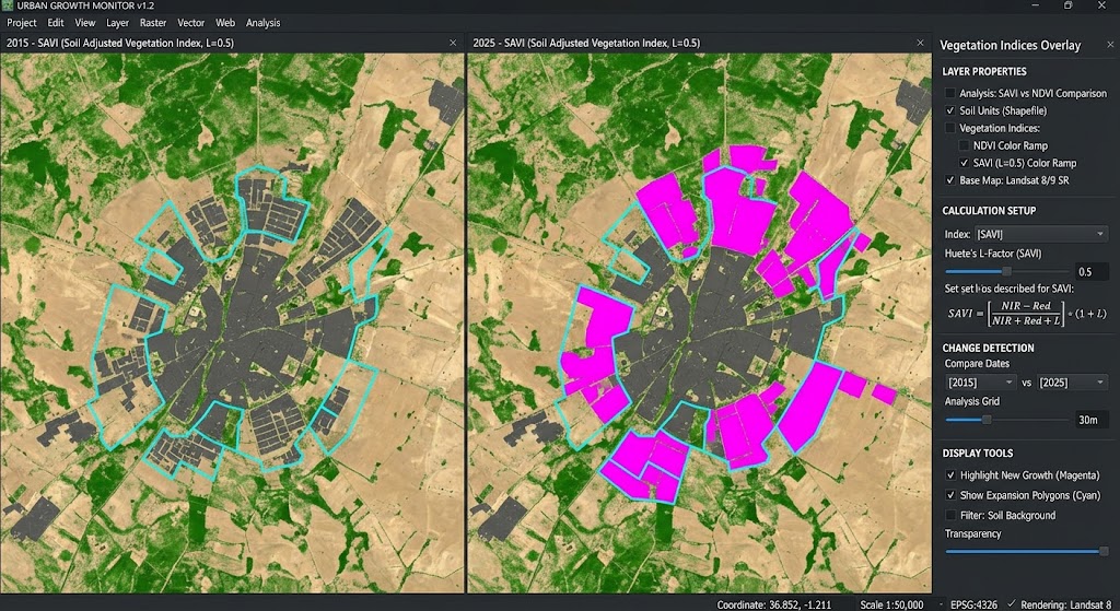
For a clearer change map, subtract the binary built-up candidate raster for 2015 from the equivalent raster for 2025.

Assuming both rasters use 1 for candidate built-up pixels and 0 for other valid land pixels, use:

"BuiltUp_2025@1" - "BuiltUp_2015@1"

Save the output as:

BuiltUp_change_2015_2025.tif

Interpret the resulting values as follows:

Difference value	Interpretation
+1	Newly classified as built-up in 2025
0	No change in the binary classification
-1	Classified as built-up in 2015 but not in 2025

Ensure that pixels marked as NoData in either year are handled consistently. Otherwise, the difference map may contain misleading results around water, clouds, or masked locations.

Style the change raster using distinct categories for new built-up candidates, unchanged areas, and areas no longer classified as built-up.

Step 12: Estimate the Area of Urban Expansion

After identifying newly classified built-up pixels, estimate the corresponding area.

For a 30-metre Landsat grid:

[
Area_{\text{pixel}}=30\times30=900\ m^2
]

This is equivalent to 0.09 hectares per pixel.

Therefore:

\text{New built-up pixels}\times0.09
]

For a 20-metre grid, each square pixel represents 400 m² or 0.04 hectares.

These calculations assume a projected grid with the stated cell dimensions and valid, consistently classified pixels. If the raster is in a geographic CRS measured in degrees, first use an appropriate projected grid or calculate area with a suitable area-aware method.

For publication-quality results, validate the mapped change using reference imagery, sample-based accuracy assessment, or a more robust land-cover classification. Report the result as estimated newly built-up area if it is based only on an NDBI threshold.

Screenshot cue: Show the final urban change map with new built-up candidates highlighted, together with a legend and the study boundary.

7. Conclusion: Environmental Implications of Urban Expansion

Calculating NDBI in QGIS provides an accessible way to explore changes in potential built-up surfaces using freely available satellite imagery.

By combining the NDBI formula with NDWI water masking, optional NDVI filtering, and multi-temporal comparison, GIS analysts can investigate the distribution and potential expansion of urban land.

The method also has important environmental applications.

Urban Heat Islands: Expansion of impervious surfaces can reduce vegetation cover and alter surface energy balance. These changes can contribute to higher surface temperatures and exacerbate urban heat-island effects, although NDBI alone does not measure temperature. Thermal imagery and appropriate surface-temperature analysis are needed to investigate this relationship.

Loss of Agricultural Land: Urban growth into peri-urban areas can convert agricultural fields and other open land into buildings and paved surfaces. A carefully validated multi-date land-cover analysis can help identify where these transitions may be occurring.

For a strong GIS university project, remember to document your satellite data sources, dates, reflectance processing, CRS, raster alignment, masking rules, thresholds, and validation method.

The central lesson is that NDBI is a useful starting point for urban expansion analysis, but reliable built-up mapping depends on more than a positive index value. Combining spectral information with careful change detection and independent validation produces more defensible conclusions about how cities are growing and how that growth affects the surrounding landscape.