
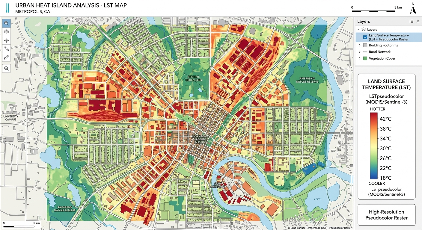
Land Surface Temperature (LST) Calculation in QGIS using Landsat 8/9
Introduction
When calculating Land Surface Temperature QGIS Landsat datasets, remember that LST is the temperature of the Earth’s surface as measured by a thermal remote-sensing sensor. Unlike air temperature measured by a weather station, LST describes the temperature of the land surface itself—for example, a road, building roof, bare soil, or vegetation canopy.
For Landsat 8 and Landsat 9, the Thermal Infrared Sensor (TIRS) provides thermal information through Bands 10 and 11. Band 10 covers approximately 10.6–11.19 µm and is commonly used for single-band LST calculations. Although the native thermal resolution is 100 m, Landsat 8/9 thermal products are delivered resampled to 30 m. USGS
The important point is that the temperature recorded by the satellite is not immediately the true land surface temperature. The original Level-1 image contains calibrated digital numbers that must first be converted to top-of-atmosphere (TOA) spectral radiance, then to brightness temperature. Surface emissivity must subsequently be estimated to account for the fact that different materials emit thermal energy differently. USGS provides the required radiometric coefficients and thermal constants in the scene’s MTL metadata file. USGS
LST is particularly useful for studying the Urban Heat Island (UHI) effect. Urban materials such as asphalt, concrete, and rooftops can become considerably warmer than vegetated or rural surfaces. By producing an LST map in QGIS, you can identify spatial patterns of surface heating and compare temperature differences between built-up areas, vegetation, water, and bare soil.
What You Need
Before beginning the Land Surface Temperature QGIS Landsat workflow, prepare the following.
1. Landsat 8 or Landsat 9 Level-1 data
For this workflow, download Collection 2 Level-1 imagery.
You need at least:
- Band 4 — Red
- Band 5 — Near Infrared (NIR)
- Band 10 — Thermal Infrared
- MTL metadata file
Landsat Collection 2 Level-1 products contain the spectral bands and an MTL metadata file containing the coefficients required to convert the digital numbers into radiance and brightness temperature. USGS
For the NDVI calculation:
NDVI = (NIR − Red) / (NIR + Red)

NDVI = (Band 5 − Band 4) / (Band 5 + Band 4)
For thermal calculations, use Band 10.
Important: Do not copy generic radiance coefficients from another Landsat scene. Use the
RADIANCE_MULT_BAND_10,RADIANCE_ADD_BAND_10,K1_CONSTANT_BAND_10, andK2_CONSTANT_BAND_10values contained in your own MTL file.
2. QGIS
Install a current version of QGIS.
You should be comfortable with:
- Loading raster layers
- Opening Raster Calculator
- Creating raster outputs
- Using layer properties
- Applying raster symbology
3. Basic raster mathematics
Most of this workflow can be performed using the QGIS Raster Calculator.
You will eventually create:
Band 10
   ↓
TOA Radiance
   ↓
Brightness Temperature
   ↓
NDVI
   ↓
Fractional Vegetation Cover
   ↓
Land Surface Emissivity
   ↓
LST
Step 1: Calculate Top-of-Atmosphere Spectral Radiance
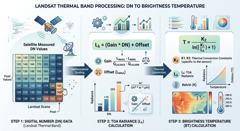
The Landsat Level-1 thermal image initially contains calibrated digital numbers (DNs). These must be converted into physical spectral radiance values.
USGS specifies the following equation for Level-1 data: USGS
TOA Radiance Formula
Lλ = ML × Qcal + ALWhere:
- Lλ = TOA spectral radiance
- ML = multiplicative radiance scaling factor
- Qcal = pixel digital number (DN)
- AL = additive radiance scaling factor
For Landsat Band 10, the metadata will contain:
RADIANCE_MULT_BAND_10
RADIANCE_ADD_BAND_10
1.1 Find the coefficients
Open the MTL file that came with your Landsat scene.
Search for:
RADIANCE_MULT_BAND_10and:
RADIANCE_ADD_BAND_10You may see values similar to:
RADIANCE_MULT_BAND_10 = ...
RADIANCE_ADD_BAND_10 = ...
Use the actual values from your scene.
1.2 Calculate radiance in QGIS
Open:
Raster → Raster Calculator
Your expression will conceptually be:
("Band10@1" × ML) + ALReplace ML and AL with the values from your MTL file.
For example, if your metadata contained hypothetical values:
ML = 0.0003342
AL = 0.1
your expression would be:
("Band10@1" * 0.0003342) + 0.1Save the result as:
B10_TOA_Radiance.tifWhy do this?
The DN is essentially a coded measurement. Radiance converts that measurement into a physical quantity describing the thermal energy detected by the sensor.
Step 2: Convert TOA Radiance to Brightness Temperature
Now that you have spectral radiance, you can convert it into brightness temperature.
Brightness temperature is the temperature a theoretical perfect emitter would need to have to produce the observed radiance.
It is not yet the final LST because the Earth’s surface is not a perfect emitter.
2.1 Brightness Temperature Formula
USGS gives the following conversion: USGS
T = K2 / ln((K1 / Lλ) + 1)Where:
- T = brightness temperature in Kelvin
- K1 = thermal conversion constant
- K2 = thermal conversion constant
- Lλ = TOA spectral radiance
- ln = natural logarithm
The MTL file contains:
K1_CONSTANT_BAND_10
K2_CONSTANT_BAND_10
Again, use the values belonging to your specific scene.
2.2 Calculate Kelvin temperature
In QGIS Raster Calculator:
K2 / ln((K1 / "B10_TOA_Radiance@1") + 1)Save this as:
Brightness_Temperature_K.tif2.3 Convert Kelvin to Celsius
Most GIS maps are easier to interpret in Celsius.
Use:
Temperature(°C) = Temperature(K) − 273.15In QGIS:
"Brightness_Temperature_K@1" - 273.15Save the result as:
Brightness_Temperature_C.tifCheck your result: A normal terrestrial scene should not suddenly produce temperatures of hundreds or thousands of degrees Celsius. Extremely abnormal values usually indicate a scaling-factor, metadata, NoData, or formula problem.
Step 3: Calculate NDVI and Fractional Vegetation Cover
Brightness temperature alone does not provide an accurate estimate of LST because different surfaces have different emissivities.
A common way to estimate emissivity is to use vegetation information derived from NDVI (Normalized Difference Vegetation Index).
3.1 Calculate NDVI
Landsat 8/9 uses:
- Band 4 = Red
- Band 5 = NIR
The NDVI equation is:
NDVI = (NIR − Red) / (NIR + Red)Therefore:
NDVI = (Band 5 − Band 4) / (Band 5 + Band 4)In QGIS Raster Calculator:
("Band5@1" - "Band4@1") /
("Band5@1" + "Band4@1")
Save it as:
NDVI.tif3.2 Interpret NDVI
A simplified interpretation is:
| Surface | Typical NDVI behavior |
|---|---|
| Dense vegetation | High positive values |
| Grass/crops | Moderate positive values |
| Bare soil | Low positive values |
| Built-up surfaces | Low or near-zero values |
| Water | Usually negative |
The exact values vary according to season, surface conditions, atmospheric effects, and preprocessing.
3.3 Calculate Fractional Vegetation Cover
Fractional vegetation cover, commonly written as Pv, estimates the proportion of vegetation within a pixel.
A widely used approach is:
Pv = ((NDVI − NDVImin) /
      (NDVImax − NDVImin))²
Where:
- Pv = fractional vegetation cover
- NDVImin = minimum NDVI for the selected scene/study area
- NDVImax = maximum NDVI for the selected scene/study area
Example
Suppose your study area has:
NDVImin = 0.05
NDVImax = 0.80
For a pixel with:
NDVI = 0.50then:
Pv = ((0.50 − 0.05) / (0.80 − 0.05))²

Pv = (0.45 / 0.75)²

Pv = 0.36
The pixel therefore has an estimated fractional vegetation cover of 0.36, or approximately 36%.
Important
Do not automatically use -1 and +1 as NDVImin and NDVImax unless your methodology specifically calls for those theoretical limits.
For a student project, it is usually better to document how you determined the minimum and maximum values for your study area.
Step 4: Estimate Land Surface Emissivity
Now we need to account for surface emissivity (ε).
What is emissivity?
Imagine two surfaces at exactly the same physical temperature:
- A dark roof
- Vegetation
They may not emit thermal radiation in exactly the same way.
Emissivity describes how efficiently a real surface emits thermal radiation compared with an ideal blackbody.
This matters because the satellite measures emitted radiation, not temperature directly.
4.1 A commonly used emissivity relationship
For a simplified NDVI-based workflow, land surface emissivity can be estimated using:
ε = 0.004 × Pv + 0.986Where:
- ε = land surface emissivity
- Pv = fractional vegetation cover
This is a commonly used empirical approximation for vegetation-based LST workflows.
4.2 Calculate emissivity in QGIS
Open Raster Calculator and enter:
(0.004 * "Pv@1") + 0.986Save the output as:
Emissivity.tifYour emissivity raster should generally contain values close to 1.
Important: This is a simplified emissivity model. More advanced LST studies may use land-cover-specific emissivity values, ASTER GED emissivity products, or atmospheric correction methods.
Step 5: Apply the Final LST Formula in Raster Calculator
Now we have the three major components needed for the simplified single-channel LST calculation:
- Brightness temperature
- Surface emissivity
- Thermal wavelength
The final step is to combine them.
5.1 Final LST formula
A commonly used single-channel correction is:
LST = BT /
      [1 + (λ × BT / ρ) × ln(ε)]
Then convert Kelvin to Celsius:
LST(°C) = LST(K) − 273.15Where:
- LST = land surface temperature
- BT = brightness temperature in Kelvin
- λ = effective wavelength of the thermal band
- ρ =
hc/σ, approximately 14,388 μm·K - ε = land surface emissivity
- ln(ε) = natural logarithm of emissivity
For Landsat 8/9 Band 10, a commonly used effective wavelength is approximately:
λ ≈ 10.895 μmBand 10 spans approximately 10.6–11.19 µm. USGS
5.2 QGIS Raster Calculator expression
Using the brightness temperature in Kelvin, your conceptual expression is:
(
  "Brightness_Temperature_K@1" /
  (
    1 +
    (
      (10.895 * "Brightness_Temperature_K@1") / 14388
    )
    *
    ln("Emissivity@1")
  )
)
) - 273.15
Save the output as:
LST_Celsius.tifImportant unit rule
Do not use Celsius in the final LST equation.
The formula requires brightness temperature in Kelvin.
The correct sequence is:
Radiance
   ↓
Brightness Temperature (K)
   ↓
Emissivity correction
   ↓
LST (K)
   ↓
LST (°C)
Creating an LST Map in QGIS
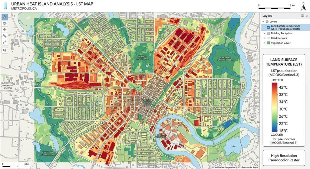
Once LST_Celsius.tif has been created, style it so that temperature patterns are easy to interpret.
1. Open Layer Properties
Right-click:
LST_Celsius → Properties → Symbology
Select:
Singleband pseudocolor
2. Choose a temperature classification
You could classify the raster into categories such as:
| LST | Example interpretation |
|---|---|
| <20°C | Relatively cool |
| 20–25°C | Moderate |
| 25–30°C | Warm |
| 30–35°C | Hot |
| >35°C | Very hot |
These are example visualization classes, not universal temperature thresholds. Your study area’s climate, season, time of acquisition, and local conditions should determine appropriate classifications.
3. Compare different land-cover types
Your final map might reveal patterns such as:
Vegetation → cooler
Water → cooler
Bare soil → warmer
Roads → warmer
Dense buildings → warmer
This is where LST becomes especially useful for Urban Heat Island GIS analysis.
Using LST to Study Urban Heat Islands
A simple UHI analysis can compare LST between different land-cover zones.
For example, divide your study area into:
- Dense urban areas
- Residential areas
- Industrial areas
- Vegetated areas
- Water bodies
- Rural/reference areas
Then calculate the mean LST for each zone.
For example:
| Land cover | Mean LST |
|---|---|
| Dense urban | 34.2°C |
| Industrial | 35.1°C |
| Residential | 31.8°C |
| Vegetation | 25.4°C |
| Water | 23.1°C |
This can reveal spatial relationships between urbanization and surface heating.
Important distinction
LST is not the same thing as air temperature.
A satellite LST map describes the temperature of the land surface, whereas conventional weather stations measure air temperature. Therefore, avoid writing that your LST map directly represents the temperature people experience.
Common Mistakes
Mistake 1: Using the wrong emissivity formula or threshold
One common error is treating emissivity as though it were a constant for every pixel.
A vegetation-covered pixel and an impervious urban pixel can have different thermal emission properties.
If you use an NDVI-based approach, make sure you correctly calculate:
NDVI
   ↓
NDVImin / NDVImax
   ↓
Pv
   ↓
ε
Also make sure your emissivity raster contains sensible values rather than zeros, negative values, or values substantially greater than 1.
Mistake 2: Mixing Kelvin and Celsius
This is one of the most important errors to avoid.
The brightness-temperature equation produces:
BT = KelvinThe final LST correction also expects:
BT = KelvinOnly after the final temperature has been calculated should you convert to Celsius:
°C = K − 273.15If you insert Celsius directly into the LST equation, your result can be severely distorted.
Mistake 3: Using the wrong metadata coefficients
Do not assume that the same radiance coefficients apply to every scene.
For each Level-1 scene, use the coefficients supplied in its MTL file. USGS specifically states that the Level-1 product metadata provides the radiometric scaling factors and thermal constants required for these conversions. USGS
Mistake 4: Using Band 11 instead of Band 10 without explaining why
Landsat 8/9 have two TIRS thermal bands. However, this tutorial uses Band 10 for the single-band workflow.
USGS identifies Band 10 as the first TIRS thermal band and notes that the historical calibration uncertainty of Band 11 has been larger; quantitative work should therefore carefully consider the calibration characteristics rather than blindly applying a two-band split-window approach. USGS
Mistake 5: Forgetting clouds and cloud shadows
Clouds can produce extremely misleading temperature values.
Before interpreting an LST map:
- Inspect the scene visually.
- Use the appropriate QA band where available.
- Mask clouds and cloud shadows.
- Exclude obvious invalid pixels.
A beautiful temperature map can still be scientifically useless if cloudy pixels are included.
Complete QGIS LST Workflow
For a quick reference, your entire workflow is:
Landsat 8/9 Level-1
        ↓
Band 10 DN
        ↓
TOA Radiance
Lλ = ML × Qcal + AL
        ↓
Brightness Temperature
T = K2 / ln((K1/Lλ) + 1)
        ↓
NDVI
NDVI = (B5 − B4) / (B5 + B4)
        ↓
Fractional Vegetation Cover
Pv = ((NDVI − NDVImin) /
      (NDVImax − NDVImin))²
        ↓
Land Surface Emissivity
ε = 0.004Pv + 0.986
        ↓
LST
LST = BT / [1 + (λBT/ρ)ln(ε)]
        ↓
Convert K → °C
LST°C = LSTK − 273.15
        ↓
LST MAP
Summary & Takeaways
Calculating Land Surface Temperature in QGIS using Landsat 8/9 is essentially a sequence of physical conversions rather than a single Raster Calculator operation.
The five major stages are:
- Convert Band 10 DN to TOA spectral radiance.
- Convert radiance to brightness temperature in Kelvin.
- Calculate NDVI and fractional vegetation cover.
- Estimate surface emissivity.
- Apply the emissivity correction to obtain LST and convert it to Celsius.
The most important formulas to remember are:
Lλ = ML × Qcal + ALBT = K2 / ln((K1 / Lλ) + 1)NDVI = (B5 − B4) / (B5 + B4)Pv = ((NDVI − NDVImin) /
(NDVImax − NDVImin))²ε = 0.004Pv + 0.986LST(K) = BT /
[1 + (λ × BT / ρ) × ln(ε)]LST(°C) = LST(K) − 273.15The key lesson is that Band 10 does not directly give you LST. You must account for radiometric scaling, brightness temperature, and surface emissivity before interpreting the result as land surface temperature.
For university GIS and remote-sensing assignments, always document your Landsat product, acquisition date, metadata coefficients, NDVI range, emissivity method, wavelength, spatial resolution, cloud masking method, and final LST formula. That makes your workflow reproducible and much easier to defend in a methodology section. USGS