
Top 5 Common Map Projections Every GIS Student Needs to Know (Plus the Distortion Trade-Offs That Decide Your Grade)
Introduction: Why You Can’t Flatten a Sphere Without Breaking Something
Whether you are preparing for a lab practical or writing a research paper, mastering common map projections GIS professionals rely on is essential for preventing costly spatial errors. Every map you have ever looked at is a lie — a useful, carefully engineered lie, but a lie nonetheless. When learning about common map projections GIS students quickly realize that the Earth is an oblate spheroid. The Earth is an oblate spheroid, a slightly squashed ball, and there is no mathematical way to peel that surface flat onto a sheet of paper or a computer screen without distorting something. This isn’t a limitation of current technology; it’s a hard geometric truth, the same reason you can’t flatten an orange peel without tearing or stretching it.
For GIS students, understanding what gets distorted — and choosing a projection that protects the property your analysis actually depends on — is one of the most important skills you’ll develop. Pick the wrong projection for a lab exercise and your area calculations will be wrong, your distances will lie, or your shapes will bulge in ways that make your map look amateurish (and cost you marks).
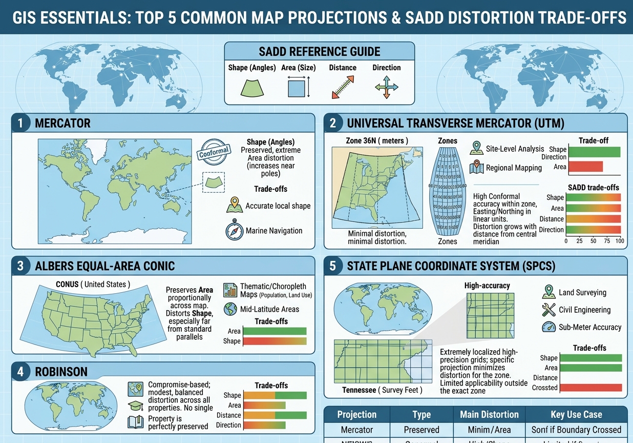
Cartographers organize this trade-off around a simple framework, often remembered by the acronym SADD:
- Shape — Are angles and local shapes preserved? (Conformal projections)
- Area — Is the relative size of regions preserved? (Equal-area projections)
- Distance — Are distances between points accurate? (Equidistant projections)
- Direction — Are compass bearings preserved? (Azimuthal properties)
No projection preserves all four simultaneously. This is known as the fundamental theorem of map projections, and it’s the reason there isn’t one “best” projection — only the best projection for your specific purpose. A navigator crossing open ocean cares about direction. A demographer comparing country populations cares about area. A surveyor platting a parcel of land cares about distance and shape at a very local scale.
Below are the five projections you’re most likely to encounter in coursework, lab exams, and real-world GIS work — what each one preserves, what it sacrifices, and when to reach for it.
1. Mercator Projection: The Navigator’s Map That Distorted the World’s Perception
The Mercator projection, developed by Flemish cartographer Gerardus Mercator in 1569, is probably the map projection you’ve seen the most — and possibly without realizing its flaws are baked into your mental image of the world. This is why the Mercator projection became one of the standard common map projections GIS courses focus on for nautical and web mapping.
Conformal Properties
Mercator is a conformal (shape-preserving) cylindrical projection. This means that at any given point, the angles between lines are preserved exactly as they appear on the globe. A 90-degree turn on your compass corresponds to a 90-degree turn on the map. This property makes small, local shapes — a coastline, a building, a city block — look geometrically correct no matter where they sit on the map.
Why Sailors Loved It
Mercator’s real genius was solving a practical navigation problem. On a Mercator map, any straight line drawn between two points represents a rhumb line — a path of constant compass bearing. A ship’s navigator could draw a straight line from origin to destination, read off a single compass heading, and sail that heading the entire way without needing to constantly recalculate direction. Before satellite navigation, this was an enormous practical advantage, and it’s why the Mercator projection became the standard for nautical charts for nearly four centuries.
The Pole Problem
The cost of this conformal property is severe area distortion that grows without bound as you approach the poles. Mercator achieves shape preservation by stretching the east-west spacing of lines of latitude further and further apart as latitude increases, to compensate for the fact that meridians (lines of longitude) converge toward the poles on a real globe but are drawn as parallel vertical lines on the flat map.
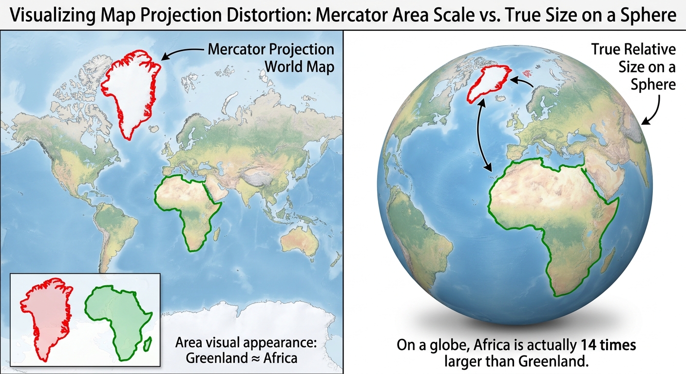
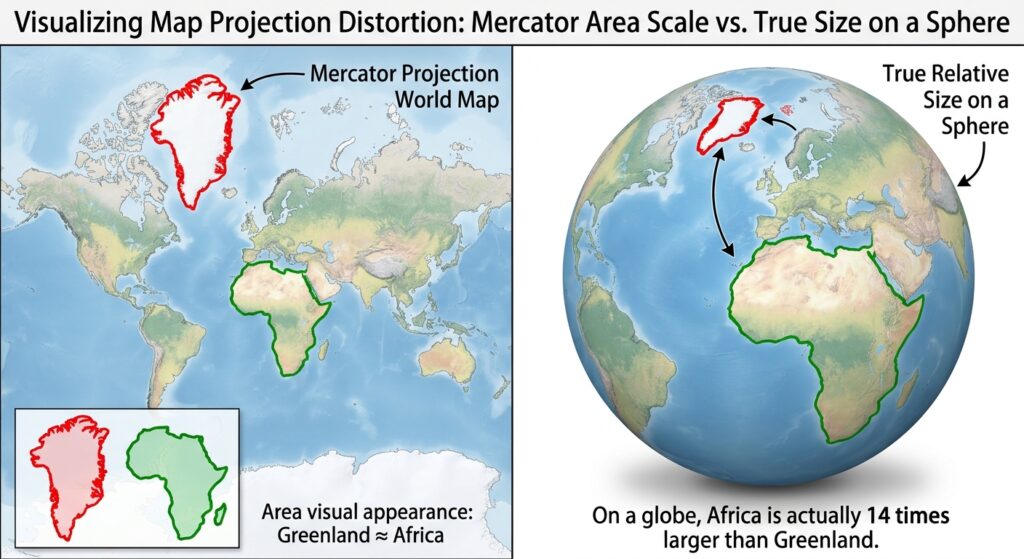
The result is the notorious “Greenland problem”: Greenland appears roughly the same size as Africa on a Mercator map, when in reality Africa is about 14 times larger. Antarctica appears as an enormous band stretching across the entire bottom of the map, when it’s actually smaller than South America. This distortion has real-world consequences — critics have argued that the Mercator projection subtly reinforces a Eurocentric, size-inflated view of high-latitude Northern Hemisphere countries relative to equatorial and Southern Hemisphere nations.
Best used for: Marine navigation, web mapping (Google Maps and most slippy web maps use a variant called Web Mercator), and any application where local shape and direction matter more than comparative area.
Avoid for: Thematic maps comparing country sizes, population density maps, or any analysis involving area calculations near the poles.
2. Universal Transverse Mercator (UTM): The GIS Workhorse
If Mercator is the projection you’ve seen the most, UTM is the projection you’ll actually work with the most once you start doing real GIS analysis.UTM is one of the most widely used common map projections GIS professionals rely on daily. Because most regional databases default to metric coordinates, learning how UTM manages scale distortion is one of the most practical requirements in any syllabus covering common map projections GIS students study.
The Zone System
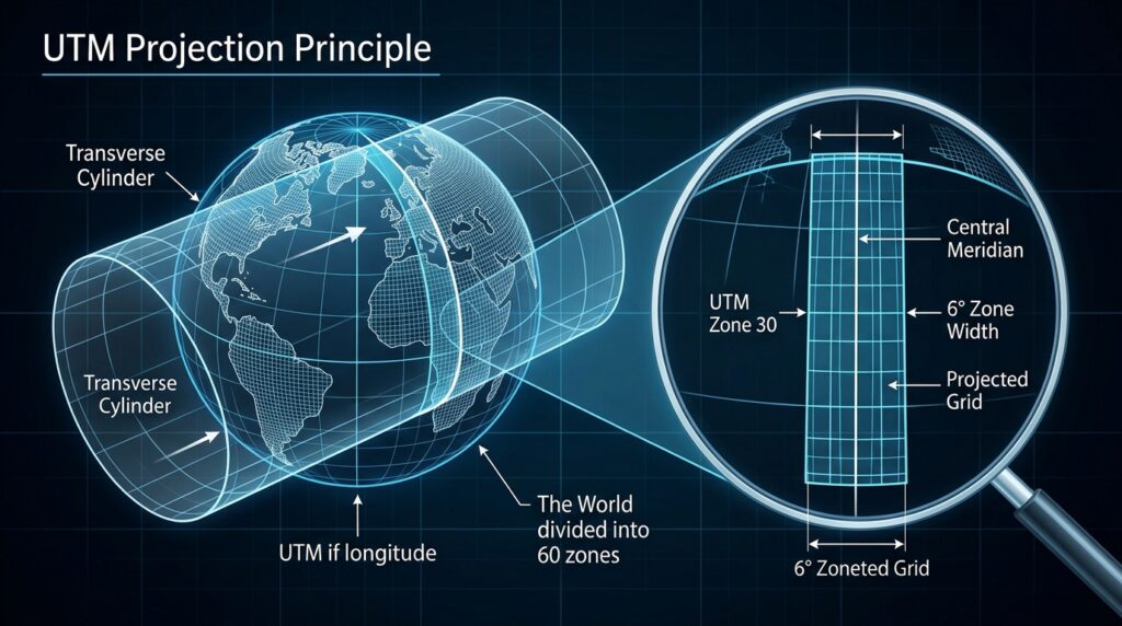
UTM solves Mercator’s distortion problem through a clever trick: instead of one cylinder wrapped around the globe touching at the equator, UTM divides the Earth into 60 narrow zones, each spanning 6 degrees of longitude. Within each zone, a transverse (sideways) cylinder is used, touching the Earth along a central meridian rather than the equator. Because each zone is narrow, the distortion within it stays minimal — generally kept below 0.04% scale error near the central meridian.
Each zone is numbered 1 through 60, starting at 180° longitude (the antimeridian) and moving eastward. Zones are further divided into latitude bands, and each hemisphere (North/South) is handled separately, since UTM uses a false northing to keep coordinates positive.
Linear Units and Practical Coordinates
Unlike geographic coordinate systems (which use degrees of latitude and longitude), UTM coordinates are expressed in meters, using an Easting and Northing value. This is enormously convenient for GIS work: because the units are linear and metric, you can directly calculate distances and areas using simple Euclidean geometry (the Pythagorean theorem) rather than the more complex spherical trigonometry required for geographic coordinates.
A typical UTM coordinate looks like: Zone 37N, 250000E, 9900000N — instantly telling you the zone, and how far east/north the point sits from a defined reference origin.
Why It’s the Gold Standard for Regional Mapping
UTM strikes an excellent balance for regional-scale work (a single country, state, or metropolitan area): it’s nearly conformal within each zone, distortion is negligible at that scale, and the metric coordinate system makes area and distance calculations straightforward without needing complex correction factors. This is why UTM is the default projection for most national mapping agencies, land surveys, and GIS datasets that don’t span multiple zones.
Best used for: Site-level and regional GIS analysis, land surveying, engineering projects, and any dataset confined to a single UTM zone (or a few adjacent ones).
Limitation: Distortion increases as you move away from the central meridian, so UTM becomes impractical for datasets spanning many zones or continental/global extents.
If calculating scale distortion or switching between zones has your lab report stalled, getting professional guidance on complex common map projections GIS modules can save you hours of trial and error.
3. Albers Equal-Area Conic: Preserving Area for Comparative Analysis
When your analysis depends on accurately comparing the size of regions — population density, land use percentages, habitat area — you need an equal-area projection, and the Albers Equal-Area Conic is the classic choice.
How Equal-Area Preservation Works
The Albers projection uses a conic projection surface — imagine a cone placed over the globe, touching (or slicing through) it along one or two lines of latitude called standard parallels. The mathematics of the projection are specifically calibrated so that any region on the map, no matter where it falls, represents the same proportional area as it does on the real globe. A 10,000 km² region in the north will occupy the same map area as a 10,000 km² region further south.
The trade-off is that shape and angles are distorted, especially far from the standard parallels. Albers minimizes this distortion by concentrating accuracy in the mid-latitudes, where the two standard parallels are typically placed.
When analyzing population distribution or land cover percentages, selecting the right equal-area framework is a core competency among the common map projections GIS analysts use to ensure equitable visual comparisons.
Why It’s Popular for Mid-Latitude Countries
The Albers Equal-Area Conic projection is the standard choice for maps of the Continental United States, largely because the country’s east-west extent and mid-latitude position align almost perfectly with the projection’s strengths. The commonly used standard parallels for the contiguous US are 29.5°N and 45.5°N, chosen specifically to minimize distortion across the country’s populated latitude range.
This same logic applies to any mid-latitude, east-west-oriented landmass — it’s frequently used for maps of Europe, China, and similar countries, always with standard parallels adjusted to that specific region.
Best used for: Choropleth maps (population density, election results, land cover), statistical and demographic analysis, and any thematic map where visually comparing region sizes matters.
Avoid for: Navigation, or any application requiring accurate local shape or direction.
4. Robinson Projection: The Diplomatic Compromise
Sometimes you don’t need any single property to be perfectly accurate — you need a map that simply looks right to a general audience. That’s the Robinson projection’s entire purpose.
Compromise Projections Explained
A compromise projection deliberately sacrifices perfect accuracy in every one of the SADD properties, distributing modest distortion across shape, area, distance, and direction rather than eliminating distortion in one category at the expense of another. The Robinson projection, developed by Arthur H. Robinson in 1963 for Rand McNally, isn’t derived from a strict mathematical formula the way Mercator or Albers are. Instead, Robinson built it by choosing coordinate values through visual trial and error, prioritizing what simply looked balanced and aesthetically pleasing.
Visual Balance Over Mathematical Purity
The result is a map where continents retain roughly recognizable, pleasing shapes, polar regions are compressed but not wildly exaggerated (unlike Mercator), and no single region looks dramatically inflated or shrunken. It’s not “correct” for any single measurement task — you shouldn’t calculate distances or areas precisely from a Robinson map — but it avoids the jarring visual distortions that make other projections look wrong to a general audience.
World Reference Mapping
Because of this balance, Robinson became the standard projection for general-purpose world maps, wall maps, atlases, and educational materials for decades. National Geographic used it as their standard world map projection from 1988 to 1998, before switching to the (also compromise-based) Winkel Tripel projection.
Best used for: General reference world maps, educational atlases, presentations, and any context where visual balance and audience readability matter more than precise measurement.
Avoid for: Any GIS analysis requiring accurate area, distance, or direction measurements — Robinson is a display projection, not an analytical one.
5. State Plane Coordinate System (SPCS): Precision at the Local Level
While UTM handles regional mapping well, some applications demand even greater precision within a smaller area. This is the niche the State Plane Coordinate System (SPCS) fills, and it’s essential knowledge if you plan to work in US surveying, civil engineering, or municipal GIS.
High-Accuracy Localized Grids
SPCS divides the United States into more than 120 numbered zones, with boundaries generally following state and county lines rather than fixed longitude bands. Each zone uses whichever projection minimizes distortion for that zone’s specific shape and orientation: Lambert Conformal Conic for states or zones that are wider east-to-west (like Tennessee), and Transverse Mercator for states or zones that are longer north-to-south (like Illinois).
Because each zone is small and the projection is chosen specifically for its geometry, SPCS achieves extremely high accuracy — distortion is generally held to less than 1 part in 10,000, far tighter than UTM’s zone-wide tolerance.
Why Engineers and Surveyors Depend on It
This level of precision matters enormously for legal land surveys, property boundary determination, and civil engineering projects, where an error of even a few centimeters can create legal disputes or construction errors. SPCS coordinates, like UTM, are expressed in linear units (historically US survey feet, increasingly meters), making distance and area calculations straightforward within a zone.
Best used for: Land surveying, cadastral (property boundary) mapping, civil engineering, construction, and any US-based project requiring sub-meter accuracy at a local scale.
Limitation: SPCS zones are small and state-specific, so it’s unsuitable for any analysis spanning multiple zones or extending beyond US borders.
Cheat Sheet: The Top 5 Map Projections at a Glance
| Projection | Type | Best Used For | Main Distortion |
|---|---|---|---|
| Mercator | Conformal | Marine navigation, web mapping | Extreme area distortion near the poles |
| UTM | Conformal (zoned) | Regional/site-level GIS, surveying | Increasing distortion away from central meridian |
| Albers Equal-Area Conic | Equal-Area | Thematic/choropleth maps, mid-latitude countries | Shape/angle distortion away from standard parallels |
| Robinson | Compromise | General world reference maps, atlases | Mild distortion spread across all properties |
| State Plane (SPCS) | Conformal (zoned) | Surveying, civil engineering, cadastral work | Minimal within zone; unusable across zones |
Conclusion: Choosing the Right Projection for Your Lab Assignment
The single most useful habit you can build as a GIS student is to ask “what property does this task actually require?” before you ever open your software’s projection dropdown menu. If you’re calculating distances or areas, you need equidistant or equal-area properties — using Mercator will silently corrupt your results even though the map “looks fine.” If you’re navigating or working with angles and bearings, you want a conformal projection like Mercator or UTM. If you’re producing a general-audience map meant to be looked at rather than measured, a compromise projection like Robinson (or its modern successors, like Winkel Tripel) will serve you better than forcing analytical accuracy where it isn’t needed.
A practical rule of thumb for coursework: default to UTM for anything site-specific or regional within a single zone, reach for Albers Equal-Area the moment your assignment involves comparing sizes or densities across regions, and remember that State Plane exists specifically for the high-precision, small-area work that surveying and engineering courses demand. Keep Mercator in your toolkit for navigation-themed exercises, and treat Robinson as a presentation tool rather than an analytical one.
Master this decision-making framework — not just the five projections themselves — and you’ll walk into your next lab exam able to justify why you chose a projection, which is exactly the kind of reasoning that separates a strong GIS answer from a merely correct one. Ultimately, knowing how to balance shape, area, distance, and direction separates a basic map from an accurate analytical product. By keeping these foundational common map projections GIS concepts in mind before you open your software’s coordinate system menu, you will ensure your spatial analysis remains both mathematically sound and visually defensible.
Struggling to finish your spatial analysis lab or tangled up in coordinate reference system errors? Don’t let projection trade-offs cost you your grade. If you need expert assistance breaking down common map projections GIS assignments require, drop a comment below or reach out to our professional support team for reliable, top-tier academic help today