Table of Contents

Multi-Criteria Evaluation GIS Site Selection: A Step-by-Step Guide

Introduction: What Is MCE in GIS?

Multi-Criteria Evaluation (MCE), also called Multi-Criteria Decision Analysis (MCDA), is a GIS-based method for combining multiple spatial criteria to identify locations that are more or less suitable for a particular purpose.

Instead of asking whether a location satisfies one condition, MCE evaluates several conditions simultaneously. For example, a solar farm site might need to have high solar radiation, gentle slopes, suitable land use, reasonable proximity to roads, and sufficient distance from protected areas.

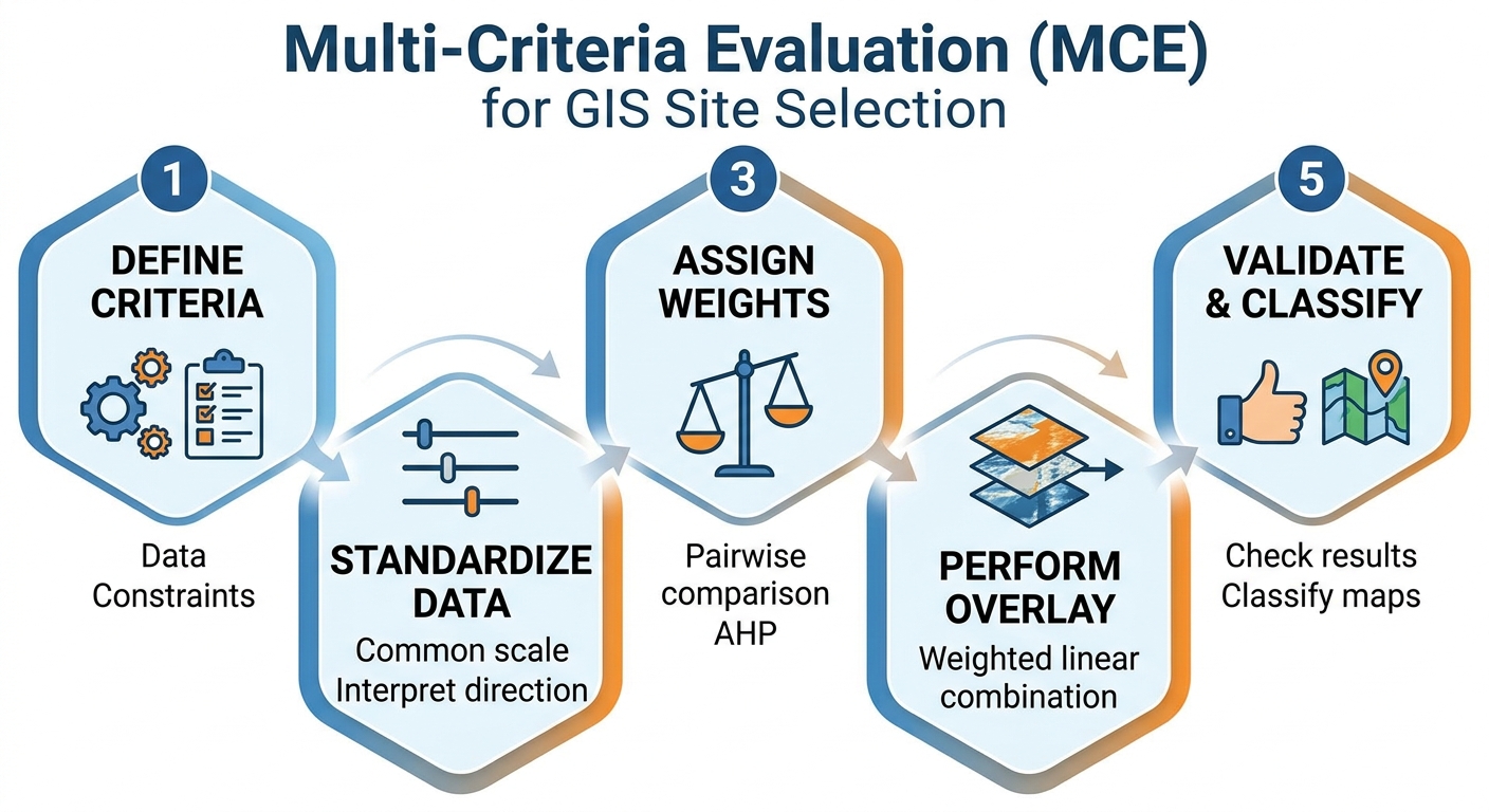
A typical multi criteria evaluation GIS site selection workflow converts these different criteria into comparable spatial scores, assigns weights according to their importance, and combines them to produce a final suitability map.

This approach is particularly useful for university GIS projects involving landfill site selection, solar farm siting, hospital location, industrial development, wind-energy planning, agricultural suitability, or conservation planning.

The central idea is:

Suitability = standardized criteria × importance weights, subject to necessary constraints.

A strong suitability analysis is therefore not simply about producing a colorful final map. You must be able to explain why each criterion was selected, how it was standardized, why each weight was assigned, how the layers were combined, and how sensitive the final result is to those assumptions.

Step 1: Define the Criteria and Gather Your Data

Before opening QGIS or ArcGIS, clearly define the decision problem.

Suppose your assignment asks you to identify suitable locations for a solar farm.

You might identify the following criteria:

Criterion	Type	Example suitability relationship
Slope	Factor	Lower slope = more suitable
Solar radiation	Factor	Higher radiation = more suitable
Distance from roads	Factor	Moderate/close distance = more suitable
Land use	Factor	Certain land uses = more suitable
Protected areas	Constraint	Exclude
Rivers	Constraint	Exclude buffer zone
Settlements	Constraint	Exclude buffer zone

This distinction between constraints and factors is fundamental.When conducting a multi criteria evaluation gis site selection project, separating factors from constraints is essential.

Constraints

.In a multi criteria evaluation gis site selection project, a constraint represents an area that is not available for the proposed development.

It is usually represented using a Boolean value:

1 = allowed
0 = excluded

For example, if environmental regulations prohibit construction inside a protected area:

Protected area
0 = unsuitable/excluded
1 = available

You can create constraints using buffers, masks, Boolean expressions, or spatial overlays.

Examples include:

Protected areas
Water bodies
Wetlands
Existing infrastructure
Legally protected zones
Hazard zones
Required setbacks from settlements

A constraint should not normally be treated as simply another factor if development there is legally or physically impossible.

Factors

A factor is a variable that influences suitability but does not necessarily eliminate an area completely.

Examples include:

Slope
Distance from roads
Elevation
Solar radiation
Soil properties
Population density
Distance from transmission lines

A factor can have different degrees of suitability.

For example:

Slope = 2° → highly suitable
Slope = 10° → moderately suitable
Slope = 25° → poorly suitable

This distinction should appear clearly in your GIS assignment methodology.

Step 2: Prepare and Standardize the Spatial Data

Your criteria will rarely use the same units.

For example:

Slope may be measured in degrees.
Distance to roads may be measured in metres.
Population density may be people/km².
Solar radiation may be measured in kWh/m².
Elevation may be measured in metres.

You cannot meaningfully add these raw values together.

A value of 500 metres does not inherently have the same meaning as 500 kWh/m².

Therefore, MCE requires standardization.

Put all criteria onto a common scale

A common approach is to convert every factor to a suitability scale such as:

1 = very unsuitable
2 = unsuitable
3 = moderately unsuitable
...
8 = suitable
9 = highly suitable
10 = extremely suitable

You could also use a 0–1 scale.

The important requirement is that all factors have the same interpretation after standardization.

Example: Reclassifying Slope

Suppose your solar farm project uses this suitability classification:

Slope	Suitability score
0–5°	10
5–10°	8
10–15°	6
15–25°	3
>25°	1

The original slope raster might contain values such as:

2.4
7.8
13.6
21.2
31.5

After reclassification, those values become:

The resulting raster is now a standardized suitability factor.

Reclassify in QGIS

In QGIS, raster reclassification can be performed using appropriate Processing tools such as Reclassify by Table.

The general workflow is:

Open the Processing Toolbox.
Search for the raster reclassification tool.
Select your slope raster.
Define the input value ranges.
Assign each range a suitability score.
Select the output data type.
Run the tool.
Inspect the resulting raster.

This is one of the most important stages in a suitability modeling tutorial because the quality of your final multi criteria evaluation gis site selection model depends heavily on how you transform raw measurements into suitability scores.

Step 3: Standardize the Direction of Suitability

Not every factor works in the same direction.

For some factors:

Higher = better

Examples:

Solar radiation
Some measures of renewable-energy potential
Certain soil-quality indicators

For others:

Lower = better

Examples:

Slope
Distance to essential infrastructure
Flood risk
Pollution exposure

Consider distance to roads.

You might decide:

0–1 km → 10
1–3 km → 8
3–5 km → 6
5–10 km → 3
>10 km → 1

The important thing is that your standardized values always have the same interpretation:

Higher score = more suitable.

Without this step, your multi criteria evaluation gis site selection weighted overlay can produce a mathematically valid but conceptually incorrect result.

Step 4: Assign Weights Using AHP

Not all criteria are equally important.

For example, a solar farm analysis might consider solar radiation more important than distance from a secondary road.

This is where the Analytic Hierarchy Process (AHP) can help.

For a multi criteria evaluation gis site selection study, AHP provides a structured method for assigning relative importance to criteria through pairwise comparison.

Instead of simply writing:

“Solar radiation is 40% important because I think it is important.”

you systematically compare criteria.

For example:

Criteria	Slope	Solar	Roads	Land use
Slope	1	1/3	2	1/2
Solar	3	1	4	2
Roads	1/2	1/4	1	1/3
Land use	2	1/2	3	1

AHP commonly uses a 1–9 importance scale, where higher values indicate that one criterion is considered more important than another.

The reciprocal is used for the opposite comparison.

For example:

Solar vs Slope = 3
Slope vs Solar = 1/3

After constructing the comparison matrix, the criteria weights can be derived and normalized so that they sum to 1 or 100%.

For illustration:

Criterion	Weight
Solar radiation	40%
Land use	25%
Slope	20%
Distance to roads	15%
Total	100%

These numbers are only an example. In an actual academic project, your weights should be supported by your research question, literature, expert justification, planning standards, or the methodology specified by your lecturer.

Why AHP strengthens a GIS assignment

AHP gives you a defensible explanation for your weights.

Instead of:

“I assigned solar radiation 40%.”

you can explain:

“Weights were derived through pairwise comparison using the AHP framework, with criteria compared according to their relative importance to solar-farm suitability.”

For a stronger methodology, report the pairwise matrix and, where appropriate, the consistency ratio used to assess whether the judgments are reasonably consistent.

Step 5: Perform the Weighted Overlay

Once your factors have been standardized and weighted, they can be combined.

The basic weighted-linear-combination model is:

$S=∑i=1nwixiS = \sum_{i=1}^{n} w_i x_i$

where:

S = final suitability score
wᵢ = weight assigned to criterion i
xᵢ = standardized suitability score for criterion i
n = number of criteria

For example:

Suitability =
(0.40 × Solar)
+ (0.25 × LandUse)
+ (0.20 × Slope)
+ (0.15 × Roads)

If every factor is standardized from 1 to 10, the resulting raster will represent relative suitability.

Weighted Overlay in ArcGIS Pro

ArcGIS Pro provides tools such as Weighted Overlay and Weighted Sum for combining raster criteria.

A typical workflow is:

Open the Spatial Analyst tools.
Locate the Weighted Overlay/Weighted Sum functionality.
Add your standardized raster layers.
Assign each layer its percentage influence.
Confirm that the evaluation scale is consistent.
Apply the analysis mask or constraints where appropriate.
Run the tool.
Inspect the output raster.

For example:

Slope suitability       → 20%
Solar suitability       → 40%
Land-use suitability    → 25%
Road suitability        → 15%

The tool calculates the combined suitability score for every raster cell.This calculation forms the backbone of any multi criteria evaluation gis site selection model

Performing the Model with Raster Calculator in QGIS

QGIS users can implement the same mathematical model using Raster Calculator.

Suppose your standardized rasters are:

solar
slope
landuse
roads

A simplified expression could be:

("solar@1" * 0.40)
+
("landuse@1" * 0.25)
+
("slope@1" * 0.20)
+
("roads@1" * 0.15)

The output is a new suitability raster.

The exact raster-band names depend on your dataset.

Applying a constraint

Suppose constraint contains:

1 = permitted
0 = excluded

You could incorporate it into the final suitability calculation:

(
("solar@1" * 0.40)
+
("landuse@1" * 0.25)
+
("slope@1" * 0.20)
+
("roads@1" * 0.15)
)
*
"constraint@1"

Areas where the constraint equals 0 will therefore receive a zero suitability value.

This demonstrates why separating factors from constraints is important.

Step 6: Check the Suitability Map

Do not immediately submit the final map. First inspect whether your multi criteria evaluation gis site selection result makes geographic sense.

Ask:

Are highly suitable areas located where you expected?
Are protected areas excluded?
Are rivers and other restricted areas properly masked?
Did a single factor dominate unexpectedly?
Are there isolated pixels that appear unrealistic?
Did all rasters use the same extent?
Do the rasters have compatible cell sizes?
Are they aligned to the same grid?

Check raster properties

Before combining rasters, make sure your datasets are compatible in terms of:

Coordinate reference system
Cell size
Extent
Alignment
NoData handling
Study-area boundary

A mismatch at this stage can produce errors or misleading results.

Step 7: Classify the Final Suitability Result

Your final continuous suitability raster for a multi criteria evaluation gis site selection project may contain values across a numerical range. For presentation, you can classify the result into categories.

such as:

Very Low Suitability
Low Suitability
Moderate Suitability
High Suitability
Very High Suitability

The exact classification method should be documented.

You could use:

Equal interval
Quantile
Natural breaks
Defined thresholds

For an academic multi criteria evaluation gis site selection project, don’t select a classification method simply because it produces the most attractive map.

Explain why the classification is appropriate for the purpose of the analysis.

Step 8: Perform Sensitivity Analysis

A strong multi criteria evaluation gis site selection analysis should acknowledge that suitability results depend on assumptions. What happens if the weights change?

Suppose your original model uses:

Solar radiation = 40%
Slope = 20%
Land use = 25%
Road distance = 15%

Create another scenario in which solar radiation receives 30% and slope receives 30%.

Then compare the results.

You might calculate:

Areas classified as highly suitable
Percentage of the study area suitable
Locations that remain suitable across scenarios
Areas whose suitability category changes

This is called sensitivity analysis.

It helps answer an important methodological question:

Are the recommended areas stable, or do they change substantially when reasonable assumptions are modified?

You don’t need to pretend that your selected weights are objectively perfect. Acknowledging uncertainty can actually strengthen an academic report.

Step 9: Writing the Methodology for Your GIS Assignment

Your methodology should allow another student to understand how you produced the final suitability map.

A useful structure is:

1. Study area

Describe:

Location
Geographic extent
Relevant environmental characteristics
Coordinate reference system

2. Data sources

Create a table such as:

Dataset	Source	Resolution/Scale	Purpose
DEM	Data source	30 m	Derive slope
Roads	Data source	—	Distance analysis
Land use	Data source	—	Land suitability
Protected areas	Data source	—	Constraint

3. Preprocessing

Explain:

Projection
Clipping
Resampling
Rasterization
Buffering
NoData handling

4. Standardization

Explain how raw values were converted to the common suitability scale.

For example:

Slope values were reclassified into five suitability classes ranging from 1 (least suitable) to 10 (most suitable).

Then provide your actual classification table.

5. Weighting

Explain how weights were derived.

For AHP, include:

Pairwise comparison matrix
Derived weights
Consistency assessment

6. Weighted overlay

Provide the mathematical model used to combine the factors.

7. Constraints

Explain which areas were excluded and why.

8. Sensitivity analysis

Describe alternative weighting scenarios and their effect on the final result.

9. Cartographic output

Include a properly designed final map containing:

Title
Legend
Scale bar
North arrow
Coordinate/grid information where appropriate
Data/source information
Author/date
Clear suitability classes

Example Methodology Paragraph

A concise methodology section might read like this:

A GIS-based Multi-Criteria Evaluation was conducted to identify suitable locations for the proposed development. Four factor layers—slope, solar radiation, land use, and distance to roads—were prepared and standardized to a common 1–10 suitability scale, where higher values represented greater suitability. Restricted areas, including protected zones and specified setback areas, were treated as Boolean constraints and excluded from the analysis. Criterion weights were derived using the Analytic Hierarchy Process through pairwise comparison. The standardized factors were subsequently combined using a weighted-linear-combination approach in a raster environment. Alternative weighting scenarios were evaluated to examine the sensitivity of the resulting suitability pattern to changes in criterion importance.

Adapt that paragraph to your actual project rather than copying it unchanged.

Common Problems in Suitability Modeling

1. Adding Raw Data Without Standardization

Combining slope degrees, distance in metres, and population density directly is inappropriate because the variables have different units and ranges.

Solution: Standardize the factors first.

2. Treating Constraints as Ordinary Factors

A legally prohibited area should not become “slightly less suitable” simply because another criterion gives it a high score.

Solution: Use a Boolean constraint or appropriate exclusion mask.

3. Assigning Arbitrary Weights

Writing “the weights were chosen because they seemed reasonable” provides weak methodological justification.

Solution: Use AHP, literature, expert consultation, planning standards, or an assignment-specified weighting scheme.

4. Ignoring CRS and Raster Alignment

Different projections, cell sizes, extents, and alignments can compromise raster analysis.

Solution: Establish a consistent raster analysis environment before performing the overlay.

5. Producing Only the Final Map

.A visually attractive multi criteria evaluation gis site selection map does not demonstrate how the result was produced.

Solution: Show your criteria, reclassification tables, weights, equations, processing workflow, and validation/sensitivity analysis.

Conclusion: Building a Strong GIS Suitability Analysis

A successful multi criteria evaluation GIS site selection project is essentially a structured decision-making workflow:

Define the problem → gather data → separate constraints and factors → preprocess → standardize → weight → overlay → validate → analyze sensitivity → map and document.

The most important lesson is that the final suitability map is only as defensible as the decisions behind it.

For a high-quality GIS capstone or suitability assignment, document where your data came from, why each criterion matters, how each criterion was reclassified, how weights were determined, how constraints were applied, and how sensitive your results are to different assumptions.

If you are working on a landfill, solar farm, hospital, agricultural, or other site-selection assignment, practice the complete workflow with a small sample dataset before processing your final study area. That makes it much easier to identify problems with raster reclassification, AHP weights, CRS settings, or weighted overlay calculations before they affect your final submission.