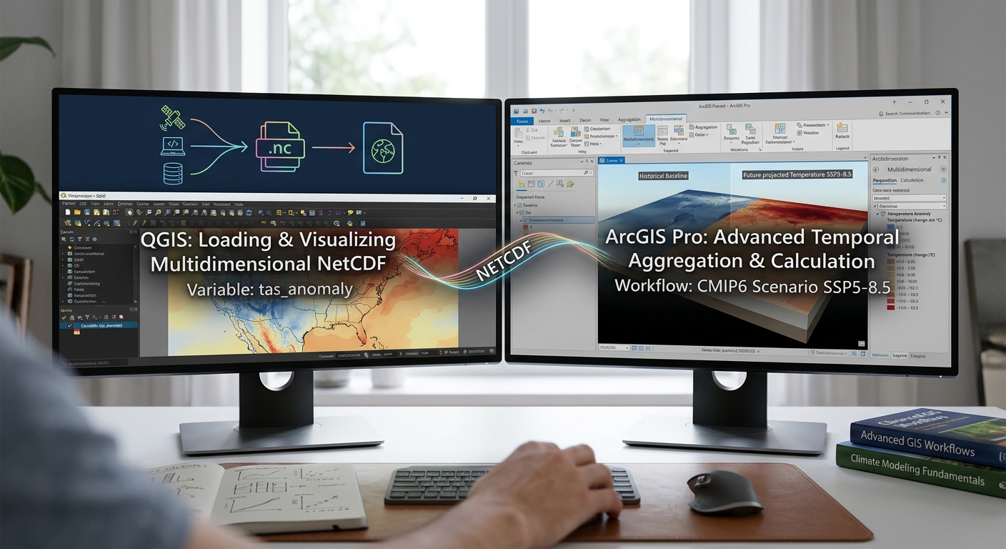
How to Map Climate Change Data: Working with NetCDF Files in QGIS & ArcGIS Pro

1. Introduction: What Are NetCDF Files and Why Are They Used in Climate Science?

To successfully Map Climate Data NetCDF QGIS ArcGIS Pro, researchers rely on large volumes of data collected or modelled across different locations and time periods. Researchers need to analyze temperature, precipitation, wind speed, sea level, and other climate variables across decades or under alternative future climate scenarios.

A common challenge is that climate data are not always delivered as ordinary GeoTIFF rasters. Many scientific datasets use the Network Common Data Form (NetCDF), typically with the .nc or .nc4 file extension.

NetCDF is a scientific data format designed to store array-based data together with descriptive metadata. It is widely used for climate and Earth system datasets because one file can contain multiple variables, spatial dimensions, time coordinates, vertical levels, and information describing how the data were produced.

For example, a NetCDF file might contain:

• Monthly mean air temperature from 1981 to 2020.
• Precipitation values for the same period.
• Latitude and longitude coordinates.
• Variable units, such as kelvin or millimetres.
• Information about the time calendar, missing values, and data source.

These capabilities make NetCDF suitable for climate research. Datasets from the Copernicus Climate Data Store, NASA Earthdata, and NOAA research archives are available in NetCDF or related scientific data formats. See the Copernicus ERA5 archive, NASA Earthdata Search, and NOAA Physical Sciences Laboratory.

The good news is that you do not need to be a climate modeller to work with NetCDF files. QGIS and ArcGIS Pro can help you inspect, visualize, extract, and analyze many NetCDF datasets through their raster and multidimensional data tools.

This tutorial follows a practical example: mapping temperature change over time, calculating annual mean temperature, and comparing future climate projections with a historical reference period.

One essential distinction comes first:

• ERA5 reanalysis provides a physically consistent reconstruction of historical weather and climate using models and observations.
• CMIP6 climate projections contain model simulations for historical experiments and possible future climate scenarios.

ERA5 is valuable for studying historical climate variability; CMIP6 is appropriate for examining possible future climate conditions under specified scenarios. They are not interchangeable datasets.

2. Understanding Multidimensional Climate Data

Before opening a NetCDF file in GIS, understand how its information is organized.When handling multidimensional matrices, researchers who Map Climate Data NetCDF QGIS ArcGIS Pro must carefully verify spatial dimensions and variable attributes

A conventional single-band raster has two spatial dimensions: rows and columns. A multidimensional climate dataset can add time, depth, elevation, model, or scenario dimensions.

2.1 Variables

A variable represents the quantity being measured or modelled.

Common climate variables include:

Variable	Common scientific name	Typical use
tas	Near-surface air temperature	Mapping temperature trends and anomalies
tasmax	Daily maximum near-surface air temperature	Studying heat extremes
tasmin	Daily minimum near-surface air temperature	Studying cold conditions and temperature ranges
pr	Precipitation flux in many CMIP datasets	Studying rainfall and projected changes
tp	Total precipitation in many ERA5 products	Mapping precipitation accumulation
uas, vas	Eastward and northward wind components	Studying wind patterns

Names vary between products, so always inspect the variable metadata rather than relying on the name alone.

For example, tas often represents temperature in kelvin, while pr in many CMIP6 datasets represents precipitation flux in kilograms per square metre per second. Total precipitation fields may instead be stored as an accumulation or depth.

These units affect the calculations you perform later.

2.2 Dimensions: Latitude, longitude, and time

Many gridded climate datasets use three primary dimensions.

• Latitude: The north–south position of each grid cell.
• Longitude: The east–west position of each grid cell.
• Time: The observation or simulation date associated with each slice.

Some datasets also include vertical levels, such as pressure levels in the atmosphere or depth levels in the ocean.

A simplified temperature dataset might look like this:

climate_data.nc
│
├── Variables
│   ├── tas       Temperature
│   └── pr        Precipitation
│
├── Dimensions
│   ├── time      January 2000 ... December 2020
│   ├── latitude  Grid rows
│   └── longitude Grid columns
│
└── Metadata
    ├── Units
    ├── Missing-value definitions
    ├── Calendar
    └── Data source

This is a conceptual example; the actual variable names, dimensions, and coordinate conventions depend on the file.

2.3 What is a time slice?

A slice is a selection of the dataset at a particular dimension value.

For temperature data, one slice might represent January 2000. Another might represent February 2000.

If the dataset contains monthly values from 2000 to 2020, the time dimension may contain 252 monthly slices.

GIS software can display selected slices, combine time steps into summary statistics, and calculate differences between periods.

A NetCDF file may expose its slices as raster bands or as multidimensional variables, depending on the data structure and software. Do not assume that every NetCDF file uses one band per month.

3. Step 1: Download a Suitable Climate Dataset

Start by deciding whether your research concerns historical conditions, climate variability, or future climate change. When downloading global scientific repositories, researchers who Map Climate Data NetCDF QGIS ArcGIS Pro must check file sizes and spatial extents carefully.

Option A: ERA5 historical climate data

The Copernicus Climate Change Service provides ERA5 reanalysis products covering decades of historical conditions.

For a beginner project, monthly mean data are often easier to manage than hourly data.

Download workflow:

• Open the ERA5 monthly averaged data on single levels.

• Register for an account and sign in if required.

• Select the appropriate product type.

• Choose a variable, such as 2 m temperature or total precipitation.

• Select the years and months required for your study.

• Define the geographic area if the data request interface supports a bounding box.

• Select NetCDF as the output format if available.

• Submit the request and download the generated file.

ERA5’s 2 m temperature represents air temperature approximately two metres above the surface. It is not the same as land surface temperature derived from satellite thermal imagery.

The ERA5 dataset documentation is available through the Copernicus Climate Data Store.

Option B: CMIP6 future climate projections

For a project about climate change, use climate model simulations from the sixth phase of the Coupled Model Intercomparison Project (CMIP6).

CMIP6 supports analysis of historical simulations and alternative future scenarios, including SSP2-4.5 and SSP5-8.5.

Download workflow:

• Open the Copernicus CMIP6 climate projections catalogue.

• Choose a variable, such as mean air temperature or daily maximum temperature.

• Select the relevant historical or future scenario.

• Define the time range, temporal resolution, and geographic coverage.

• Review the available model and ensemble information.

• Download the dataset in NetCDF format where available.

• Record the model, scenario, period, variable, and units in your research notes.

CMIP6 projections are conditional on the climate model, scenario, and assumptions used. An SSP scenario is not a prediction that one particular future must occur. See the Copernicus CMIP6 dataset documentation.

Other useful sources

Repository	Best suited to	Access
Copernicus Climate Data Store	ERA5 and CMIP6 datasets	CDS
NASA Earthdata	Satellite observations and Earth science datasets	Earthdata Search
NOAA Physical Sciences Laboratory	Gridded climate and reanalysis datasets, many in NetCDF	NOAA PSL Data
Earth System Grid Federation	Climate model outputs, including CMIP6 holdings	ESGF data access

Before downloading a global dataset, restrict its geographic and temporal extent wherever possible. A smaller file is usually easier to inspect, process, and visualize.

4. Step 2: Import NetCDF Data into QGIS

QGIS can read many NetCDF datasets using GDAL, while its mesh provider can load supported NetCDF files that contain mesh-structured data. To successfully Map Climate Data NetCDF QGIS ArcGIS Pro using raster subdatasets, always verify the layer properties and band order.

These are two different workflows. Most regular gridded climate rasters should initially be opened through the raster workflow, while mesh datasets should be loaded as mesh layers.

4.1 Load a NetCDF raster

• Open QGIS and create a new project.

• Select Layer → Add Layer → Add Raster Layer.

• Browse to your .nc file and open it.

• If QGIS identifies multiple subdatasets, select the required variable, such as tas or tp.

• Add the selected variable to the map canvas.

• Right-click the layer and open Properties → Information or Properties → Source to inspect the raster dimensions, extent, coordinate reference system, and band count.

A NetCDF file is a container and may contain several variables. QGIS may therefore ask which subdataset you want to load. This behaviour is documented in the QGIS data formats guide.

If you do not see the variable you expect, inspect the NetCDF metadata or try loading it through the Browser panel.

4.2 Load a NetCDF mesh

Use the mesh workflow when the dataset has a mesh structure supported by QGIS.

• Open Layer → Add Layer → Add Mesh Layer, or use the Mesh tab in the Data Source Manager.

• Browse to the supported NetCDF file.

• Add the mesh layer.

• Open the mesh layer properties.

• Inspect the available dataset groups and select the temperature, precipitation, or other quantity you want to display.

• Review the available symbology and temporal settings.

Mesh data may store values on vertices, edges, or faces rather than on a conventional regular raster grid. The available operations depend on the file structure and provider. See the QGIS mesh documentation.

4.3 Understand the band structure

If the selected raster layer contains multiple bands, check the band metadata to determine what each band represents.

For instance:

Band 1 = January 2000 temperature
Band 2 = February 2000 temperature
Band 3 = March 2000 temperature
...

This is only an example. The band order must be confirmed from the dataset metadata; it should not be guessed from the file name.

If the NetCDF uses a time dimension that QGIS exposes through multiple bands, you may be able to use QGIS’s temporal settings to associate bands with date ranges. To do this, open Layer Properties → Temporal and look for Fixed Time Range Per Band when supported by the layer.

That setting helps animate the data through time, but it does not itself calculate annual averages.

5. Step 3: Import NetCDF Data into ArcGIS Pro

ArcGIS Pro supports conventional NetCDF raster layers and multidimensional raster layers. For datasets containing many time steps or additional dimensions, the multidimensional workflow is generally the more flexible option. Successfully executing temporal selections when you Map Climate Data NetCDF QGIS ArcGIS Pro requires understanding time slices and coordinate reference systems.

5.1 Add the climate data

• Open your ArcGIS Pro project.

• Click Map → Add Data and browse to your NetCDF file, if supported by the data source.

• Alternatively, use Analysis → Tools and search for Make Multidimensional Raster Layer.

• Select the input NetCDF dataset.

• Specify the variable you want to analyze.

• Review the available dimensions, including time and spatial coordinates.

• Choose the required dimension values or time interval if a subset is needed.

• Run the tool and inspect the resulting layer in the Contents pane.

The Make Multidimensional Raster Layer tool can select variables and slices by dimension values, ranges, or iterations. See the official tool reference.

For a basic single-slice raster, the Make NetCDF Raster Layer tool is another option. However, Esri recommends the multidimensional tool for enhanced capabilities when analyzing multidimensional data. See Reading NetCDF as a raster layer.

5.2 Inspect the dimensions

After the dataset loads:

• Open the layer’s properties.

• Review the multidimensional information and variable names.

• Identify the dimension that corresponds to time.

• Check the available time values and their frequency.

• Confirm whether the layer represents monthly, daily, or hourly data.

If the variable contains time slices, ArcGIS Pro may expose a Multidimensional contextual tab when the layer is selected. Use the available display controls to inspect particular slices.

Important: A raster layer may initially display only one slice even when the NetCDF contains hundreds of time steps. That does not mean the other data are missing; you may need to select the intended time dimension or create a multidimensional raster layer.

6. Step 4: Extract Specific Time Steps or Date Ranges

Temporal selection allows you to focus the analysis on a particular year, season, or climate period. When extracting temporal subsets, students learning how to Map Climate Data NetCDF QGIS ArcGIS Pro should confirm the time dimension encoding.

For example, you might compare mean temperature during 1981–2010 with mean temperature during 2041–2070.

6.1 Extract time slices in QGIS

The precise method depends on how QGIS and GDAL expose your NetCDF data.

For a raster with time represented as bands:

• Confirm the time represented by each band using metadata.

• Open Raster → Conversion → Translate (Convert Format) or the corresponding GDAL processing algorithm.

• Select the desired input raster.

• Specify the band or bands corresponding to your target period, if the tool exposes band selection.

• Save the output to a new raster file.

• Repeat for additional time steps if required.

For interactive exploration, you can instead configure Layer Properties → Temporal when your raster source exposes suitable time information.

For a mesh dataset:

• Open the mesh layer properties.

• Inspect its temporal settings and available dataset groups.

• Configure the time range or dataset selection.

• Use temporal navigation to view the desired time period.

A time filter controls what is displayed. For quantitative temporal analysis, ensure the tool processes the intended slices rather than merely hiding unwanted dates in the map.

6.2 Extract time slices in ArcGIS Pro

For a multidimensional raster:

• Select the multidimensional layer or open Analysis → Tools.

• Search for Make Multidimensional Raster Layer.

• Select the input multidimensional raster.

• Choose the required variable.

• Set Dimension Definition to the appropriate option, such as By Values for particular times or By Ranges for a date range.

• Select the time dimension, such as StdTime, if that is the dimension name exposed by the dataset.

• Specify the desired date or range and run the tool.

If you need a standalone raster for one specific date, configure the tool to create a dimensionless single-slice result where that option is available. Save the result to disk if it needs to persist beyond the current session.

For ordinary NetCDF variables, the available dimension names and date formats depend on the source file. Always use the dimension values presented by the tool instead of assuming all files use the same time encoding.

7. Step 5: Calculate Annual Mean Temperature

One of the most common climate GIS tasks is calculating annual mean temperature from monthly or daily data.

Suppose your NetCDF contains monthly mean air temperature. You want to create an annual mean temperature raster for a selected year.

7.1 Understand the calculation

A simple annual mean from 12 monthly mean values is:

[
T_{\text{annual}}=\frac{T_1+T_2+\cdots+T_{12}}{12}
]

Here, each (T_i) is the mean temperature for month (i).

For more precise temporal averages, monthly means can be weighted by the number of days represented in each month. If you have daily mean temperature, calculating the mean across valid daily values is often preferable.

This distinction matters because months have different lengths, and missing values can also affect the final result.

Before calculating the mean, inspect the variable’s units. Many climate models store air temperature in kelvin. To convert Kelvin to degrees Celsius, subtract 273.15:

[
T_{^\circ C}=T_K-273.15
]

A temperature difference or anomaly can be calculated in either kelvin or degrees Celsius because the interval between the two scales is identical. For a map intended for a general audience, degrees Celsius are usually easier to interpret.

7.2 Calculate the annual mean in QGIS

One practical GUI method is to create raster slices for the relevant months and use the Raster Calculator.

• Extract the 12 monthly mean rasters for the target year.

• Confirm that all rasters use compatible grids, extents, and NoData settings.

• Open Raster → Raster Calculator.

• Enter an expression that averages the 12 monthly layers.

• Set the output extent, resolution, and destination file.

• Run the calculation and inspect the result.

For example, if the monthly layers have been saved separately:

(
  "temperature_jan@1" +
  "temperature_feb@1" +
  "temperature_mar@1" +
  "temperature_apr@1" +
  "temperature_may@1" +
  "temperature_jun@1" +
  "temperature_jul@1" +
  "temperature_aug@1" +
  "temperature_sep@1" +
  "temperature_oct@1" +
  "temperature_nov@1" +
  "temperature_dec@1"
) / 12

Replace these example layer names with the exact names shown in your QGIS Raster Calculator.

This expression assumes all 12 months are valid and that missing cells have been handled consistently. For precise monthly-to-annual calculations, especially with NoData cells or different numbers of valid days, use an appropriate temporal aggregation method that accounts for valid observations.

If your NetCDF exposes monthly slices as bands rather than separate raster layers, you can also use band-specific raster references in the calculation. Verify the band order first.

7.3 Calculate annual means in ArcGIS Pro

For a multidimensional raster containing monthly temperature slices, ArcGIS Pro can aggregate the time dimension.

• Open Analysis → Tools.

• Search for Aggregate Multidimensional Raster.

• Select the input multidimensional raster.

• Choose the temperature variable.

• Set the dimension to the time dimension, commonly StdTime.

• Choose an annual aggregation definition.

• Choose Mean as the aggregation method.

• Configure NoData handling and the output path.

• Run the tool and inspect the resulting multidimensional raster.

The tool can combine slices along a specified dimension. For instance, monthly data can be aggregated to annual intervals. See Esri’s Aggregate Multidimensional Raster documentation.

This tool is designed for multidimensional raster analysis and may require the relevant Spatial Analyst or Image Analyst licensing, depending on the workflow and tool version.

7.4 What about annual precipitation?

Do not apply the temperature averaging formula to precipitation automatically.

If the data represent monthly precipitation totals, annual precipitation is commonly calculated by summing the monthly totals. If the variable represents a precipitation rate or flux, you must account for the units and time interval before summing or converting it to a depth.

For example, a precipitation flux in kg m⁻² s⁻¹ cannot be interpreted directly as a monthly rainfall depth without accounting for the duration. Since 1 kg m⁻² of liquid water corresponds to 1 mm of water depth, the appropriate unit conversion must incorporate the time represented by the variable.

Always check the dataset’s variable metadata and documentation before calculating annual totals.

8. Step 6: Map Climate Anomalies Using Diverging Color Ramps

A climate anomaly measures how much a value differs from a defined reference condition.

For example, if annual mean temperature in 2050 is 1.8°C above a historical baseline, the temperature anomaly is +1.8°C.

An anomaly map often communicates climate change more clearly than a map of absolute temperature because it emphasizes how much a location differs from the baseline.

8.1 Calculate the anomaly

The basic calculation is:

[
\text{Anomaly}=\text{Value of interest}-\text{Reference mean}
]

Suppose your baseline is mean annual temperature during 1981–2010 and your comparison period is 2041–2070.

For a simple illustration:

Location	Baseline mean (°C)	Future mean (°C)	Anomaly (°C)
Area A	24.0	25.5	+1.5
Area B	21.0	22.2	+1.2
Area C	19.5	19.0	−0.5

These are illustrative values, not observed or projected results for a specific region.

The anomaly calculation should compare like with like. If you are examining future change using CMIP6 data, a defensible method is to compare the future period with an appropriate historical simulation from the same model and data processing framework, where available.

8.2 Style anomalies in QGIS

• Open the anomaly raster’s Properties → Symbology.

• Select Singleband pseudocolor.

• Choose a diverging color ramp with a neutral midpoint.

• Set the minimum, midpoint, and maximum deliberately.

• Center the color ramp at zero when the intended interpretation is positive versus negative change.

• Label the legend with the anomaly units, such as °C.

• Check that NoData areas are not shown as zero anomalies.

A useful palette might use blue for negative anomalies, a pale neutral colour around zero, and red for positive anomalies.

The actual range should reflect the data. Do not force extreme values into a misleading colour distribution simply to make the map more visually striking.

8.3 Style anomalies in ArcGIS Pro

• Select the anomaly raster.

• Open Raster Layer → Symbology.

• Choose Stretch for continuous anomaly values where appropriate.

• Select a diverging colour scheme.

• Adjust the stretch range so that zero is the meaningful midpoint.

• Confirm that the legend title and units are correct.

• Inspect the output at the final map scale.

For a classified anomaly map, you may instead use meaningful intervals, such as below −2°C, −2 to −1°C, −1 to 0°C, 0 to 1°C, 1 to 2°C, and above 2°C, if those thresholds are appropriate for the study.

8.4 Create a historical-versus-future comparison

A strong climate mapping project can show three outputs:

1. A historical baseline temperature map.
2. A future period temperature map.
3. A temperature anomaly map showing the difference.

This gives readers both the absolute climate conditions and the change relative to the baseline.

When comparing CMIP6 projections, document the model, scenario, baseline period, future period, variable, units, and any downscaling or bias correction applied.

A single model and scenario do not represent the full uncertainty in future climate. If your research allows, compare several models or an ensemble and communicate the range of results.

9. Common Beginner Errors to Avoid

Before finalizing your climate map, check the following:

Error 1: Treating ERA5 as a future projection. ERA5 is a reanalysis dataset. Use climate model projections such as CMIP6 when the question concerns possible future climate conditions.

Error 2: Assuming every NetCDF file has the same structure. Variables, dimensions, calendars, and band layouts vary between files. Inspect the metadata first.

Error 3: Mixing units. Confirm whether temperature is stored in kelvin or degrees Celsius and whether precipitation is stored as a total, depth, or rate.

Error 4: Confusing visual time filtering with temporal analysis. Animating a NetCDF layer does not calculate annual means or climate anomalies. Use an appropriate aggregation or raster calculation tool.

Error 5: Comparing unrelated scenarios or models without explanation. Ensure the baseline and future datasets are compatible and document the model, period, and scenario.

Error 6: Interpreting map colours as certainty. A projected anomaly describes modelled change under particular assumptions. It is not a guarantee of the exact future value at a location.

Error 7: Ignoring NoData and the calendar. Some climate datasets use calendars such as noleap or 360_day. Confirm that the GIS workflow handles the time dimension correctly, especially when extracting specific date ranges and aggregating to annual values.

10. Summary: Building a Reproducible Climate GIS Workflow

Working with NetCDF files becomes manageable once you understand the relationship between variables, spatial coordinates, and time dimensions. Following these structured workflows allows students to Map Climate Data NetCDF QGIS ArcGIS Pro with high accuracy and reproducible results. Following these steps enables analysts to Map Climate Data NetCDF QGIS ArcGIS Pro efficiently and produce reproducible climate maps.

A defensible workflow follows these steps:

1. Download the right dataset from a repository such as Copernicus, NASA Earthdata, NOAA, or ESGF.
2. Inspect the metadata to understand the variables, dimensions, units, time coordinates, and grid.
3. Load the appropriate variable into QGIS or ArcGIS Pro using the raster, mesh, or multidimensional tools that match the file structure.
4. Extract the relevant dates or slices and calculate temporal summaries using methods appropriate to the data.
5. Calculate anomalies using a clearly defined reference period.
6. Visualize results with meaningful colour ramps and units.
7. Document the analysis so that another researcher can reproduce the result.

For university climate or environmental GIS assignments, start with a manageable monthly dataset and a well-defined study area. Once you can load a variable, inspect its dimensions, calculate an annual mean, and produce a meaningful anomaly map, you will have established the foundations for more advanced climate analysis.

The key is to move beyond treating NetCDF as just another raster file. It is a structured scientific dataset whose time dimension, units, and metadata are essential to interpreting the climate patterns shown on your map.