
LiDAR Data in GIS: 5 Steps to Create Digital Surface Models (DSM)
Introduction
LiDAR (Light Detection and Ranging) is a remote-sensing technology that measures the distance between a sensor and objects on the Earth’s surface using laser pulses. A LiDAR survey can produce millions of three-dimensional points containing X, Y, and Z coordinates, where X and Y represent horizontal position and Z represents elevation. These measurements are commonly stored as LAS or LAZ point-cloud files, making LiDAR an important source of high-resolution elevation data for GIS analysis.
In point cloud GIS workflows, each LiDAR return can represent a different surface feature. Some points may represent bare ground, while others represent trees, buildings, vehicles, or other objects above the ground. LiDAR data therefore provides much more information than a conventional elevation raster because individual measurements can be examined and classified before generating derived surfaces.
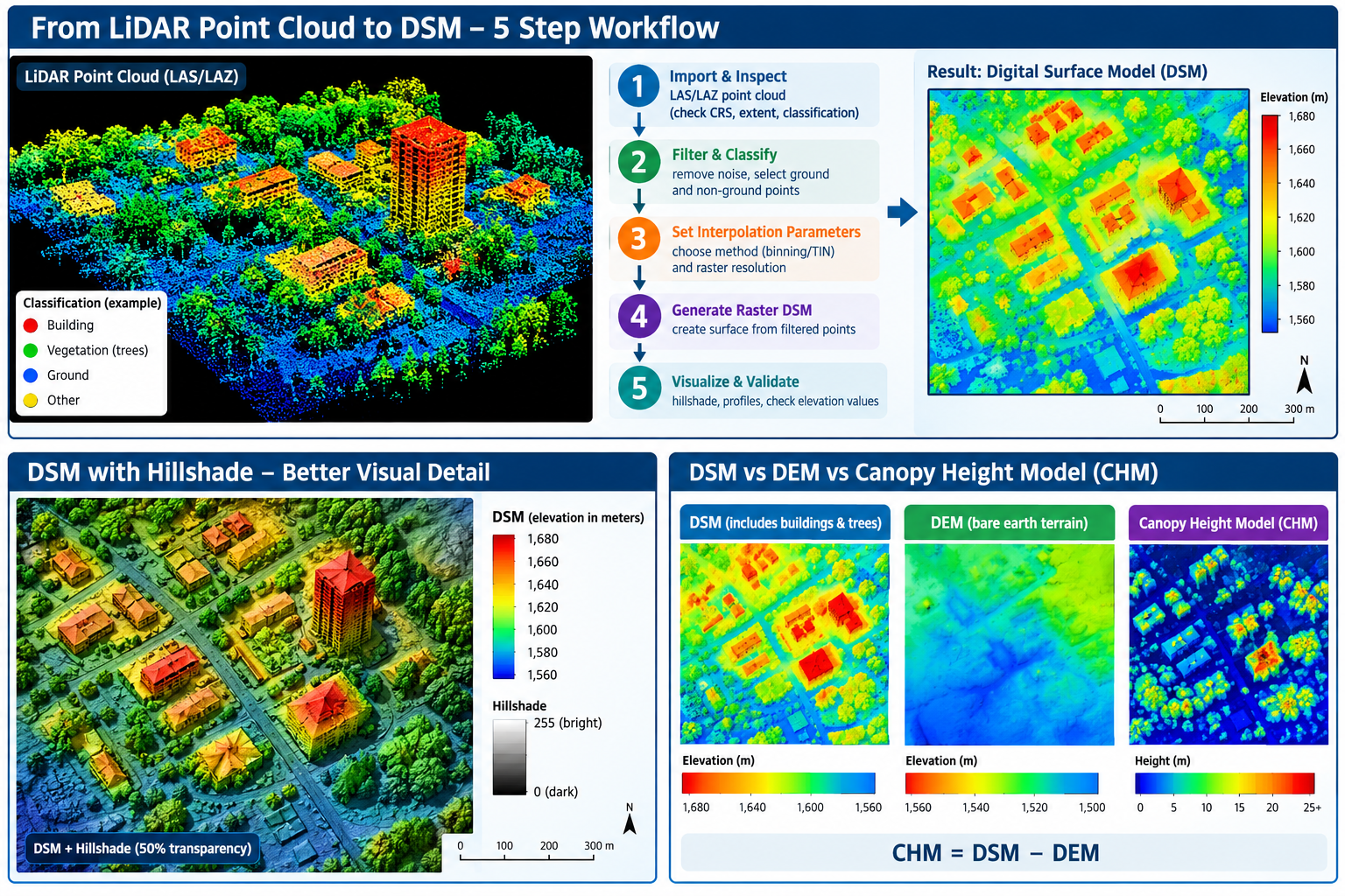
A Digital Surface Model (DSM) represents the elevation of the Earth’s surface including objects located above the ground, such as buildings, trees, bridges, and other structures. A Digital Elevation Model (DEM), in contrast, is generally intended to represent the bare-earth terrain. For example, if a 20-meter-tall building stands on terrain at 1,000 meters elevation, a DSM may contain an elevation close to 1,020 meters over the building, while a bare-earth DEM would remain close to 1,000 meters.
This distinction makes DSMs particularly useful for urban modeling, forestry, telecommunications, solar analysis, and 3D visualization. In this tutorial, you will learn a five-step workflow for turning LiDAR point-cloud data into a raster DSM using GIS software.
Prerequisites
Before starting this Digital Surface Model tutorial, prepare the following:
Software
You can complete the workflow using:
- QGIS — particularly useful for students because it is free and open source.
- ArcGIS Pro — useful if your university provides an Esri license.
- A computer with enough storage and RAM to process LiDAR data.
LiDAR dataset
You need a LAS or LAZ file.
Free LiDAR datasets are available from sources such as:
- USGS EarthExplorer
- USGS 3D Elevation Program (3DEP)
- Government open-data portals
- National mapping agencies
- University research repositories
For US-based coursework, USGS EarthExplorer is a useful starting point for finding LiDAR and elevation datasets.
Other useful data
For a university assignment, also obtain:
- A boundary polygon for your study area
- A suitable basemap
- The coordinate reference system (CRS) used by your LiDAR dataset
- Optional aerial imagery for visual validation
Tip: Start with a small LiDAR tile rather than downloading an entire county or city. LiDAR datasets can contain millions or even billions of points.
Step 1: Import and Inspect LAS/LAZ Point Cloud Files
The first stage is bringing the LiDAR point cloud into your GIS environment and determining what information it contains.
1.1 Understand LAS and LAZ
The two formats you are most likely to encounter are:
- LAS — standard binary format for LiDAR point-cloud data.
- LAZ — compressed version of LAS designed to reduce file size.
Both can contain information such as:
| Attribute | Purpose |
|---|---|
| X | Horizontal coordinate |
| Y | Horizontal coordinate |
| Z | Elevation |
| Classification | Identifies ground, vegetation, buildings, etc. |
| Intensity | Strength of the returned laser signal |
| Return number | Identifies the position of a return within a pulse |
| Number of returns | Total returns from a laser pulse |
The classification field becomes especially important later because it can help distinguish ground from vegetation and buildings.
1.2 Load the point cloud in QGIS
In QGIS:
- Open your project.
- Select Layer → Add Layer → Add Point Cloud Layer.
- Browse to your
.LASor.LAZfile. - Select the file and click Add.
- Zoom to the point-cloud layer.
Depending on the QGIS version and installed components, point-cloud tools may appear under the Processing Toolbox or point-cloud layer controls.
1.3 Inspect the point cloud
Before processing, investigate:
- Coordinate reference system
- Minimum and maximum elevation
- Point density
- Classification information
- Number of points
- Extent of the dataset
- Whether the dataset contains multiple return types
A useful first question is:
Does the dataset already contain classified ground and non-ground points?
If it does, you can usually move more quickly to DSM generation.
Step 2: Filter Noise and Classify Ground vs. Non-Ground Points
Raw LiDAR data may contain points that do not represent meaningful terrain or objects.
These can include:
- Atmospheric or sensor noise
- Isolated points
- Water returns
- Temporary objects
- Incorrectly classified measurements
Filtering improves the reliability of the resulting surface.
2.1 Understand LiDAR classification
LiDAR datasets frequently use standardized classification codes.
Common examples include:
| Classification | Typical meaning |
|---|---|
| 1 | Unclassified |
| 2 | Ground |
| 3 | Low vegetation |
| 4 | Medium vegetation |
| 5 | High vegetation |
| 6 | Building |
| 7 | Low noise |
The exact classes available depend on the dataset.
Ground vs. non-ground
For a DSM, you generally want to preserve above-ground objects such as:
- Trees
- Buildings
- Poles
- Bridges
- Other structures
For a bare-earth DEM, you would instead isolate the ground class.
This is one of the most important conceptual differences between a DSM and DEM.
2.2 Filtering the point cloud
If your LiDAR dataset is already classified, use its classification information to filter points.
For example:
DSM:
Ground + vegetation + buildings + other valid above-ground returns
DEM:
Ground points only
If the dataset is not classified, you may need to use a LiDAR classification algorithm before generating your surface.
Important
Do not automatically delete every point classified as “unclassified.” Some datasets use classification schemes differently, so inspect the dataset documentation first.
Step 3: Set Interpolation Parameters — Binning or Triangulation
A LiDAR point cloud consists of individual measurements, while a DSM raster consists of regularly spaced cells.
You therefore need a method for converting the irregular point cloud into a continuous surface.
Two common approaches are binning and triangulation.
3.1 Binning
With binning, the study area is divided into regular grid cells.
For example:
LiDAR points

 •     •
    •       •
 •       •
       •

        ↓

Raster grid

+---+---+---+
|   | • |   |
+---+---+---+
| • | • | • |
+---+---+---+
|   | • |   |
+---+---+---+
The points falling within each cell are combined according to a selected statistic.
For a DSM, a maximum elevation approach is often useful because the highest return within a cell may represent the top of a tree or building.
3.2 Choosing raster resolution
Your cell size should be related to the LiDAR point density.
For example:
- Very dense LiDAR → smaller cells may be appropriate.
- Lower-density LiDAR → larger cells may produce a more stable surface.
Avoid choosing an extremely small pixel size simply because the LiDAR dataset is high resolution.
A 0.1-meter raster does not automatically contain 0.1-meter spatial information if the underlying point density cannot support it.
3.3 Triangulation
Another approach is TIN (Triangulated Irregular Network) interpolation.
A TIN connects LiDAR points into triangular surfaces.
It can be useful where you want the surface to follow irregularly distributed elevation measurements rather than forcing all measurements into regular grid cells.
Binning vs. triangulation
| Method | Advantage | Common application |
|---|---|---|
| Binning | Simple and efficient | Large raster DSMs |
| TIN | Preserves irregular point geometry | Detailed terrain/surface modeling |
For a university assignment, document why you selected your method and cell size rather than simply reporting the software’s default settings.
Step 4: Generate the Raster DSM Layer
Once the LiDAR points have been filtered and your interpolation parameters are established, you can generate the DSM.
4.1 DSM workflow in QGIS
Depending on your QGIS version and available processing providers, tools may include point-cloud rasterization or other point-cloud processing algorithms.
The general workflow is:
- Select the LAS/LAZ point cloud.
- Select the appropriate elevation/Z attribute.
- Choose the points you want to include.
- Select a raster resolution.
- Choose the aggregation/interpolation method.
- Specify the output extent.
- Select an output raster format such as GeoTIFF.
- Run the process.
Your output should be a raster in which each cell contains an estimated surface elevation.
4.2 Check the resulting raster
After processing, inspect:
- Raster dimensions
- Cell size
- Minimum elevation
- Maximum elevation
- NoData areas
- CRS
- Spatial extent
Open the raster’s Layer Properties and check whether its CRS matches the source LiDAR data.
What should your DSM look like?
A DSM of an urban area should generally show higher values over:
- Buildings
- Trees
- Towers
- Elevated structures
Lower values should occur over:
- Roads
- Bare ground
- Open fields
- Other low surfaces
Step 5: Visualize and Validate Elevation Values
Creating a DSM is not the final step. You should verify that the output makes spatial and numerical sense.
5.1 Apply a hillshade
A hillshade converts elevation differences into simulated illumination and shadow.
This can make subtle variations in the DSM easier to recognize.
In QGIS, use a hillshade tool from the raster-processing tools and experiment with:
- Azimuth
- Altitude
- Z-factor
You can place the hillshade beneath the DSM and adjust the DSM’s transparency to create a visually informative map.
5.2 Inspect elevation values
Use the raster’s Identify Features tool to click individual DSM cells.
Record values from locations such as:
- Open ground
- Building roofs
- Tree crowns
- Roads
Compare these values with your expectations.
For example, if the surrounding terrain is approximately 1,500 m and a building is approximately 20 m tall, the DSM should show values around 1,520 m over the building roof.
5.3 Create an elevation profile
An elevation profile is another useful validation technique.
Draw a line across your study area and examine how elevation changes along the line.
A profile crossing a building might resemble:
Elevation
   ^
   |              ______
   |             |      |
   |_____________|      |________
   |
   +-----------------------------> Distance
The sudden increase represents the building height above surrounding terrain.
A forested area may show many smaller fluctuations caused by individual trees.
5.4 Compare DSM and DEM
If you also have a bare-earth DEM, subtract it from the DSM:
Canopy/Structure Height = DSM − DEM
This produces a height-above-ground surface.
For example:
| Location | DSM | DEM | DSM − DEM |
|---|---|---|---|
| Open ground | 1,500 m | 1,500 m | 0 m |
| Building | 1,518 m | 1,500 m | 18 m |
| Tree canopy | 1,527 m | 1,500 m | 27 m |
This difference raster is the foundation for a LiDAR canopy height model (CHM).
Practical Use Cases
1. Forestry Canopy Analysis
One of the most common applications of a LiDAR DSM is measuring vegetation structure.
A workflow could be:
DSM − DEM → Canopy Height Model → Tree/Forest Analysis
The resulting LiDAR canopy height model can help identify:
- Tree height
- Canopy structure
- Forest gaps
- Vegetation density
- Areas of tall vegetation
- Potential forest disturbance
For example, if a DSM contains tree-top elevations while a DEM represents bare ground, subtracting the DEM from the DSM provides an estimate of vegetation height.
Student project idea
Select a forested study area and:
- Generate the DSM.
- Obtain or generate a DEM.
- Calculate
DSM - DEM. - Symbolize the resulting CHM.
- Identify areas containing vegetation taller than a selected threshold.
2. Urban Building Height Estimation
DSM data can also be used to investigate urban structures.
Buildings appear as elevated surfaces in a DSM. If you have a bare-earth DEM, you can calculate:
Building/Surface Height = DSM − DEM
This can help estimate:
- Building height
- Roof elevation
- Urban morphology
- Development density
- Potential solar exposure
- 3D city characteristics
For more advanced analysis, building footprints can be combined with the height raster to calculate statistics for individual buildings.
Common Troubleshooting Problems
Problem 1: The LAS file has no CRS or the CRS appears incorrect
A missing or incorrect coordinate reference system can cause the point cloud to appear in the wrong location.
Solution
Check the metadata supplied with the LiDAR dataset.
Do not guess the CRS based only on how the layer looks. Confirm the coordinate system from the dataset documentation or metadata and assign the correct CRS before performing spatial analysis.
Problem 2: The LiDAR file is extremely large
High-density point clouds can contain millions of points and consume substantial RAM and disk space.
Solution
Start with a small tile or clip the point cloud to your study area.
You can also:
- Process tiles separately.
- Reduce unnecessary point density where appropriate.
- Use LAZ compression for storage.
- Avoid creating unnecessarily tiny raster cells.
- Save intermediate outputs to a drive with sufficient free space.
Tip: If QGIS becomes unresponsive, the dataset may simply be too large for your computer rather than technically incorrect.
Problem 3: The DSM contains holes or strange elevation spikes
Gaps can occur when there are insufficient LiDAR returns in an area. Spikes may result from noise or incorrectly classified points.
Solution
Inspect the original point cloud and classification data.
Check:
- Noise classes
- Point density
- Missing returns
- Interpolation settings
- Cell size
- Maximum/minimum elevation statistics
Do not immediately fill every gap with interpolation because doing so can create artificial elevation values.
Conclusion
Creating a DSM from LiDAR Data in GIS involves more than simply converting a LAS file into a raster. A reliable workflow requires you to understand the point cloud, inspect its classification, remove or filter problematic points, choose an appropriate interpolation method, and validate the resulting elevation surface. When completing university lab assignments, applying LiDAR data in GIS ensures high-precision surface modeling and accurate spatial analysis.
The five-step workflow can be summarized as:
- Import and inspect the LAS/LAZ point cloud.
- Filter and classify ground and non-ground points.
- Set interpolation parameters such as cell size and binning or triangulation.
- Generate the raster DSM.
- Visualize and validate the elevation surface using hillshade, profiles, and point inspection.
Once you understand this workflow, you can move beyond basic DSM creation into more advanced applications such as forest canopy height modeling, building-height estimation, urban 3D analysis, and terrain-surface comparison.
Frequently Asked Questions
What is the difference between a DSM and a DEM?
A DSM represents the elevation of the surface including above-ground objects such as trees and buildings. A DEM generally represents the bare-earth terrain.
Can QGIS open LAS and LAZ files?
Yes. Modern QGIS versions provide support for LiDAR point clouds, including common LAS/LAZ datasets. Processing capabilities can vary depending on the QGIS version and installed processing providers.
What is a LiDAR canopy height model?
A Canopy Height Model (CHM) represents the height of vegetation above the ground. A common method is:
CHM = DSM − DEM
The result can be used to estimate tree and vegetation heights.
Should I use binning or triangulation?
It depends on your project. Binning is straightforward for creating raster products from dense point clouds, while triangulation/TIN can preserve irregular point distributions. For most introductory raster DSM assignments, binning is a practical starting point.
Why is my DSM much larger than my DEM?
That is expected where buildings, trees, or other structures are present. The DSM records the top of those features, whereas the DEM represents the underlying terrain.