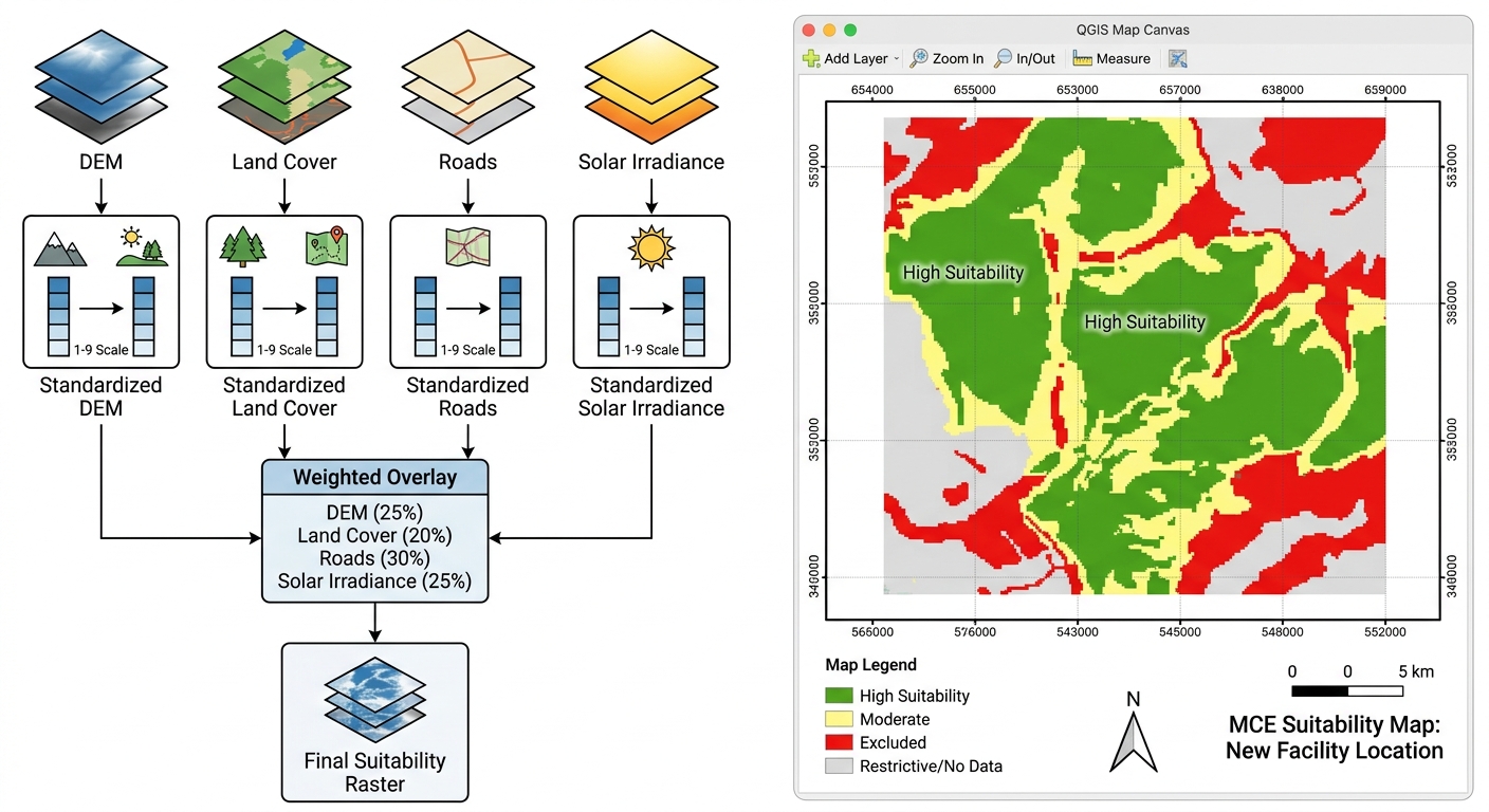
Site Suitability Analysis using Multi-Criteria Evaluation (MCE) in GIS

A practical workflow for university GIS projects using QGIS and ArcGIS Pro

Site suitability analysis is one of the most useful applications of GIS because it helps researchers identify locations that best meet a set of environmental, economic, technical, and social requirements.

This guide follows a hypothetical solar farm site-selection project to explain the complete workflow, from choosing criteria to producing and validating a suitability map.

The central idea is simple: prepare geographic data representing different site-selection criteria, standardize those criteria onto a common scale, assign relative importance to each factor, and combine them into a final suitability surface—while excluding locations where development is not permitted.

Introduction: What Is Multi-Criteria Evaluation in GIS?

Multi-Criteria Evaluation (MCE) is a structured method for evaluating locations against several criteria simultaneously. When combined with GIS, it allows spatial data to be compared and integrated to identify areas that are more or less suitable for a particular purpose.

For example, a proposed solar farm may require:

• Relatively flat terrain to reduce construction complexity.

• High solar irradiation to support electricity generation.

• Reasonable access to roads and electrical infrastructure.

• Suitable land cover that avoids sensitive ecosystems.

• Separation from legally protected areas and other restricted locations.

No single dataset can answer all these questions. A solar-resource map may identify areas with excellent sunshine, but some of those locations may be too steep, difficult to access, or environmentally restricted.

MCE combines these different considerations into a spatial decision model.

The process follows a widely used GIS-based multi-criteria decision analysis approach: transform the criteria to a common scale, then weight and combine them. See Esri’s Multicriteria Overlay documentation.

The same principles apply to landfill placement, hospital location planning, wind farms, conservation prioritization, and other spatial decision problems. The criteria and exclusion rules must change to suit each application.

Phase 1: Criteria Selection and Constraint Identification

The first stage is deciding which geographic conditions make a location suitable and which conditions automatically disqualify it.

This distinction is fundamental to a reliable MCE model.

Step 1.1: Define the objective and study area

For this example, assume the objective is:

Identify potentially suitable locations for a utility-scale solar farm within a defined county or planning region.

Before processing data, document the basic requirements:

• Define the study area boundary.
• Specify the type and approximate size of facility being considered.
• Establish the required map resolution and geographic scale.
• Identify environmental, engineering, planning, and legal requirements.
• Decide what constitutes a high-suitability result.

A rooftop solar installation and a utility-scale solar farm have different spatial requirements. A useful model must reflect the type of facility being evaluated.

Step 1.2: Identify factors

A factor is a condition that affects how suitable a location is. Its influence can vary across the study area rather than simply classifying every location as acceptable or unacceptable.

For a solar farm, possible factors include slope, solar irradiation, distance to roads, and land cover.

The relationships above are examples, not universal engineering rules. Some facilities require a minimum road setback, for example, even though access to roads is desirable. That setback should be treated as a separate constraint when appropriate.

Practical advice: Avoid including several highly correlated factors without justification. For instance, road distance and distance to electricity infrastructure may partly represent the same accessibility advantage. Giving both excessive weight can unintentionally count the same consideration twice.

Step 1.3: Identify constraints

A constraint is a condition that excludes a location from consideration, regardless of how well it scores on other factors.

Possible solar-farm constraints include:

• Protected areas where the proposed development is prohibited.

• Water bodies and wetlands, including applicable protection buffers.

• Legally restricted zones.

• Existing built-up areas where construction is not permitted.

• Areas exceeding a clearly justified engineering limit.

• Land subject to other binding planning restrictions.

For example, a protected wetland should not become an acceptable candidate simply because it has excellent solar irradiation and convenient road access.

This is why constraints should be separated from suitability factors.

In raster analysis, constraints are often represented by a Boolean mask: one value identifies eligible cells, and another identifies excluded cells. Alternatively, excluded areas can be assigned NoData or an explicit restricted value supported by the analysis tool.

Important: Use applicable legislation, official protected-area boundaries, planning requirements, and documented technical standards to set exclusions. A student suitability model is a preliminary screening tool, not a substitute for environmental assessment, land-rights checks, engineering surveys, or regulatory approval.

Phase 2: Data Preparation and Standardization

Once the criteria are defined, prepare the input datasets so that they can be combined correctly.

The central task is to convert the different inputs into spatially aligned raster layers with comparable suitability scores.

Step 2.1: Collect and inspect the input data

For a solar-farm exercise, gather:

• A study-area boundary polygon.
• A DEM for calculating slope.
• A solar-resource raster.
• A road-network dataset.
• A land-cover dataset.
• Protected-area and other exclusion-zone boundaries.

Inspect the source, date, scale or resolution, CRS, data quality, and intended use of each dataset.

Possible sources include government mapping agencies, official land-cover products, trusted elevation datasets, and documented solar-resource datasets.

Step 2.2: Standardize the coordinate system and raster grid

Raster overlay requires careful alignment. Two rasters can appear to overlap on the map while their pixel grids are offset from each other.

Before combining rasters:

• Reproject the input data into a suitable projected CRS for the study area.
• Choose a common cell size appropriate to the data and decision scale.
• Set a common processing extent.
• Align pixel origins and grids using a reference or snap raster.
• Check NoData handling and ensure that all output rasters cover the intended study area.

The chosen cell size should reflect the coarsest meaningful source data and the intended decision scale. Resampling a 100 m source to 10 m does not create genuine 10 m detail.

For more on raster alignment, see the QGIS raster tools documentation.

Step 2.3: Convert vector data to raster where necessary

Weighted raster overlay requires criteria to be represented on a compatible raster grid. Not all inputs begin in raster format, so you may need to derive or convert some datasets.

Slope from a DEM

• In QGIS, open the Processing Toolbox and locate the Slope algorithm under terrain analysis.

• In ArcGIS Pro, use Slope in the Spatial Analyst or relevant raster-analysis tools.

• Save the result in a suitable raster format and inspect its units, such as degrees or percent rise.

Land cover from polygons

• In QGIS, use Rasterize (vector to raster) through the Processing Toolbox.

• In ArcGIS Pro, use Polygon To Raster.

• Use an appropriate categorical field to encode land-cover classes.

• Ensure the raster cell size, extent, and alignment match the other analysis rasters.

Do not treat categorical class codes such as 1, 2, and 3 as suitability scores automatically. Those numbers may simply be identifiers for forest, grassland, and urban land. Reclassify them according to your documented criteria.

Distance to roads

A road network is usually converted into a distance raster rather than simply rasterizing road locations.

• In QGIS, use a suitable proximity or distance algorithm.

• In ArcGIS Pro, use Distance Accumulation or an appropriate Euclidean-distance tool.

• Confirm the units and whether the distance is straight-line or network-based.

For local site screening, straight-line distance may be adequate for an initial model. Road-network travel distance may be more appropriate when accessibility depends on the actual transport network.

Step 2.4: Create exclusion buffers

Some constraints are based on proximity rather than just the location of a feature itself.

For example, the planning framework may require a buffer around particular water bodies or sensitive facilities.

• Identify the features requiring protection or separation.
• Confirm the relevant buffer distance from official requirements or a documented study assumption.
• Use the Buffer tool on the relevant vector layers.
• Combine the resulting exclusion areas with other constraints.
• Convert or rasterize the exclusion zones to align with the analysis grid if your workflow uses raster overlay.

Do not use arbitrary buffer distances simply because they produce a visually neat map. Every buffer should have a defensible source or be explicitly identified as a modelling assumption.

Step 2.5: Reclassify factors onto a common suitability scale

The input datasets contain different measurements:

• Slope may be measured in degrees.

• Distance to roads may be measured in metres.

• Solar irradiation may be measured in energy per unit area over a defined period.

• Land cover may contain categorical codes.

You cannot meaningfully add these raw values together without standardizing what they represent.

Reclassification converts original values into a common scale, such as 1–9, where:

• 1 represents very low suitability.

• 9 represents very high suitability.

The direction must be set separately for each factor. For slope, a smaller number of degrees may receive a higher suitability score. For solar irradiation, higher values may receive a higher score. Distance criteria may favour locations closer to roads, subject to any required exclusion buffer.

Here is an illustrative reclassification table for a hypothetical solar-farm model.

These thresholds are illustrative only. Actual limits must be determined from technical requirements, site conditions, and the project’s purpose. The best road-distance range may not be the closest range if access buffers, safety, or other requirements apply.

Use similarly documented scoring tables for solar irradiation and land cover. For categorical land cover, explicitly state which categories are preferred, less preferred, or excluded.

In QGIS:

• Open the Processing Toolbox.
• Search for Reclassify by Table.
• Select the raster band to reclassify.
• Enter the minimum and maximum ranges and their new suitability scores.
• Assign NoData to categories that should be excluded from the factor raster, where appropriate.
• Save each reclassified raster.

See the QGIS Reclassify by Table documentation.

In ArcGIS Pro:

• Open Analysis → Tools.
• Search for Reclassify.
• Choose the input raster and the field or values to reclassify.
• Specify the new suitability values.
• Save the output raster.

At the end of this stage, every factor should have a clearly documented meaning, a common evaluation scale, and the same aligned raster grid.

Phase 3: Weight Assignment and Overlay Analysis

Now that the factor rasters use a common scale, the next question is how much importance each factor should contribute to the final result.

A slope requirement may be more important for one development than road accessibility. A conservation model may prioritize habitat integrity above access to roads. The weights encode these priorities.

Step 3.1: Choose a method for assigning weights

There are several ways to assign criteria weights.

Equal weighting: Give every factor the same weight. This is simple and useful as a baseline, but it assumes all criteria matter equally.

Expert judgment: Assign weights based on technical knowledge, stakeholder priorities, published standards, or a documented planning framework.

Analytic Hierarchy Process (AHP): Use pairwise comparisons to judge the relative importance of each criterion and derive weights systematically.

AHP is commonly applied to GIS suitability analysis because it provides a structured way to convert expert preferences into numerical weights. It also includes a consistency check to help identify contradictory comparisons. See this GIS–AHP site-suitability study.

Step 3.2: Assign example weights

For this hypothetical solar-farm project, suppose the criteria are weighted as follows:

These weights are demonstration values, not recommended weights for every solar-farm project. You should justify your own values using technical evidence, stakeholder requirements, or a documented decision process.

The weights must sum to 100% for the classic ArcGIS Pro Weighted Overlay tool. For formulas using decimal weights, the equivalent total is 1.0.

Step 3.3: Use pairwise comparison with AHP

In AHP, you compare the criteria in pairs. For example:

• How much more important is solar irradiation than slope?

• How much more important is slope than road access?

• How important is land-cover compatibility relative to solar irradiation?

A common AHP judgment scale ranges from 1 to 9:

Intermediate values can express judgments between these levels. The reverse comparison uses the reciprocal value.

Once the pairwise matrix is complete, calculate the priority weights and assess consistency. A commonly used guideline is a Consistency Ratio (CR) below about 0.10, although interpretation depends on the method and context. If the ratio exceeds that level, review the judgments for contradictions rather than accepting the weights automatically.

For a student project, you can use a documented AHP calculator or spreadsheet and include the comparison matrix, final weights, and consistency result in an appendix.

Step 3.4: Calculate the weighted suitability score

The weighted linear combination method calculates a score for every eligible raster cell by multiplying each standardized factor by its weight and adding the results.

Conceptually:

Where:

• \(S\) is the final suitability score.

• \(w_i\) is the weight of criterion \(i\).

• \(x_i\) is the standardized suitability score for that criterion.

• \(n\) is the number of criteria.

For the four-factor example:

Here, \(R\) is the solar-resource score, \(T\) is the terrain score, \(A\) is the road-access score, and \(L\) is the land-cover score.

Suppose a cell has these values:

Because all four factor scores use the same 1–9 scale and the weights sum to 1.0, the combined score remains on that general scale. A score of 7.65 indicates relatively favourable conditions under these particular assumptions, not a universal probability of success.

Step 3.5: Run Weighted Overlay in ArcGIS Pro

ArcGIS Pro’s classic Weighted Overlay tool combines integer rasters that have been reclassified to a common suitability scale. Each raster receives a percentage influence, and the percentages must sum to 100. The tool also supports a restricted value for excluding locations. See the Weighted Overlay tool documentation.

Use the following procedure:

• Ensure that the factor rasters are integer rasters and use a compatible evaluation scale.
• Open Analysis → Tools.
• Search for Weighted Overlay.
• Select the evaluation scale supported by your chosen workflow.
• Add the reclassified factor rasters.
• Enter their percentage influences.
• Check that the percentages total 100.
• Configure remap values and restricted values as required.
• Set the processing extent, cell size, and alignment environments.
• Choose an output raster and run the tool.

The classic Weighted Overlay tool requires the relevant Spatial Analyst capability. If your workflow needs floating-point output or decimal weights without integer rounding, consider an appropriate weighted-sum or raster-calculator approach instead.

Step 3.6: Calculate the weighted overlay in QGIS

QGIS provides reclassification and raster-calculator workflows for combining suitability rasters. For example, if the standardized raster layers are named solar_suit, slope_suit, road_suit, and landcover_suit, the weighted expression is:

0.35 * "solar_suit@1" +
0.25 * "slope_suit@1" +
0.20 * "road_suit@1" +
0.20 * "landcover_suit@1"

To run it:

• Open Raster → Raster Calculator or search for Raster Calculator in the Processing Toolbox.
• Insert each raster layer using the layer and band names displayed by QGIS.
• Enter the weighted expression.
• Set the output extent and cell size consistently with the input rasters.
• Save the output to a file rather than relying only on a temporary layer.
• Inspect the resulting statistics and suitability pattern.

The expression assumes all input rasters have already been reclassified to a common scale and aligned correctly.

Apply the constraint mask separately so restricted cells are excluded from the candidate areas. In QGIS, you can use a raster mask or an appropriate raster-calculator condition to preserve only eligible cells; do not let excluded cells silently contribute as if they were ordinary low-suitability values.

Why constraints should not simply receive a low score

Weighted overlay is an additive model. A location with a poor score on one factor can still receive a high overall score if the other factors are favourable.

That compensation is acceptable for some preferences, but it is inappropriate for a legal exclusion. A protected area must remain excluded even if all the other criteria score highly.

Therefore, apply the exclusions as a separate mask or supported restricted-value rule and verify that they remain excluded in the final output.

Phase 4: Output Sensitivity and Validation

A suitability map is the result of a model, not an unquestionable statement about the real world. The output depends on the selected data, classifications, weights, and exclusions.

This final phase tests whether the candidate areas remain reasonably consistent when assumptions change and checks whether the results are plausible.

Step 4.1: Classify the suitability raster

After producing the weighted score raster, classify the result into meaningful categories.

For example:

These classes are illustrative and should be adapted to the output’s actual score distribution and the purpose of the project. If a weighted-sum calculation produces fractional values, choose break points that suit the resulting range.

In QGIS, style the output with Singleband pseudocolor or another appropriate raster renderer. In ArcGIS Pro, use Classify or Classified raster symbology, as appropriate to the output.

Use a restrained colour ramp that makes high and low suitability easy to distinguish. Make sure the excluded areas remain visibly distinct from areas that are merely low-scoring.

Step 4.2: Perform sensitivity analysis

Sensitivity analysis tests how much the model’s results change when its assumptions are adjusted.

For example, your initial model might assign a 20% weight to road access. You could run additional scenarios that assign it 10% and 30%, adjusting the other weights so that the total remains 100%.

• Run the original model with the documented weights.
• Create one or more alternative, plausible weighting scenarios.
• If justified, test alternative reclassification thresholds or distance cutoffs.
• Compare the high-suitability zones between scenarios.
• Record whether the same candidate areas remain prominent or the results change substantially.

If a candidate location remains highly suitable across several reasonable scenarios, that may suggest that the result is relatively robust to the tested assumptions. If it disappears whenever a single weight changes slightly, the conclusion is more sensitive and should be reported accordingly.

Do not choose the scenario simply because it produces the most attractive or extensive suitable area.

Step 4.3: Validate the result

Validation checks whether the resulting map is reasonable given independent evidence and actual site conditions.

For a solar-farm project:

• Compare candidate areas with known environmental restrictions and official land-use information.
• Check that protected zones and required exclusion buffers are absent from the selected sites.
• Review terrain and access conditions against source data or reliable reference maps.
• Consult relevant planning, environmental, and engineering information.
• Where possible, conduct field verification or a more detailed site investigation.
• Document uncertain inputs and limitations.

A site may score highly in the raster model but still be unsuitable because of land ownership, grid-connection cost, local planning rules, biodiversity impacts, or geotechnical conditions that were not represented.

For a thesis: Record the input datasets, resolution, CRS, reclassification tables, weights, constraint criteria, overlay formula, validation methods, and sensitivity results. This makes the model reproducible and allows another researcher to understand why the candidate areas were selected.

Step 4.4: Extract and compare candidate sites

The suitability raster identifies locations, but a real development usually needs contiguous areas large enough for the proposed facility.

• Select the high-suitability class or a defensible score threshold.
• Convert eligible high-scoring raster cells to polygons if needed.
• Dissolve or group adjacent cells into candidate zones.
• Remove patches that are too small for the intended facility, using a justified minimum-area requirement.
• Inspect the candidate polygons on the map alongside constraints and reference layers.
• Rank the remaining candidates using additional project requirements where appropriate.

The final output should present the strongest candidate areas, but it should also show enough information for a reviewer to understand how they were identified.

Conclusion: Key Takeaways for Student Projects

Site suitability analysis using Multi-Criteria Evaluation combines different spatial datasets into a consistent, documented decision model.

The essential stages are:

1. Select criteria and constraints that reflect the actual decision problem.

2. Prepare the data with a suitable CRS, consistent raster grids, appropriate distances and buffers, and documented reclassification scores.

3. Assign weights and combine factors using a justified method such as expert weighting or AHP.

4. Apply hard exclusions so legally or environmentally restricted locations cannot become suitable through a high weighted score.

5. Test sensitivity and validate the results before interpreting the map or recommending candidate sites.

The most important lesson is that a suitability model is only as defensible as its assumptions. Clear criteria, justified weights, consistent data preparation, and careful validation matter more than producing a colourful final raster.

For a university assignment, aim to show not just where the model identifies suitable areas, but also why those areas score highly, which assumptions influence the outcome, and what further checks would be required before a real-world decision.

Further reading

• Esri: How Weighted Overlay Works — common evaluation scales, weights, and raster combination.

• Esri: Multicriteria Overlay — alternative overlay methods and criteria standardization.

• QGIS: Reclassify by Table — converting raster ranges to standardized class values.

• QGIS: Raster Tools — raster alignment and grid preparation.

• GIS–AHP Site Suitability Study — an example of pairwise comparisons and consistency assessment in spatial suitability modelling.