
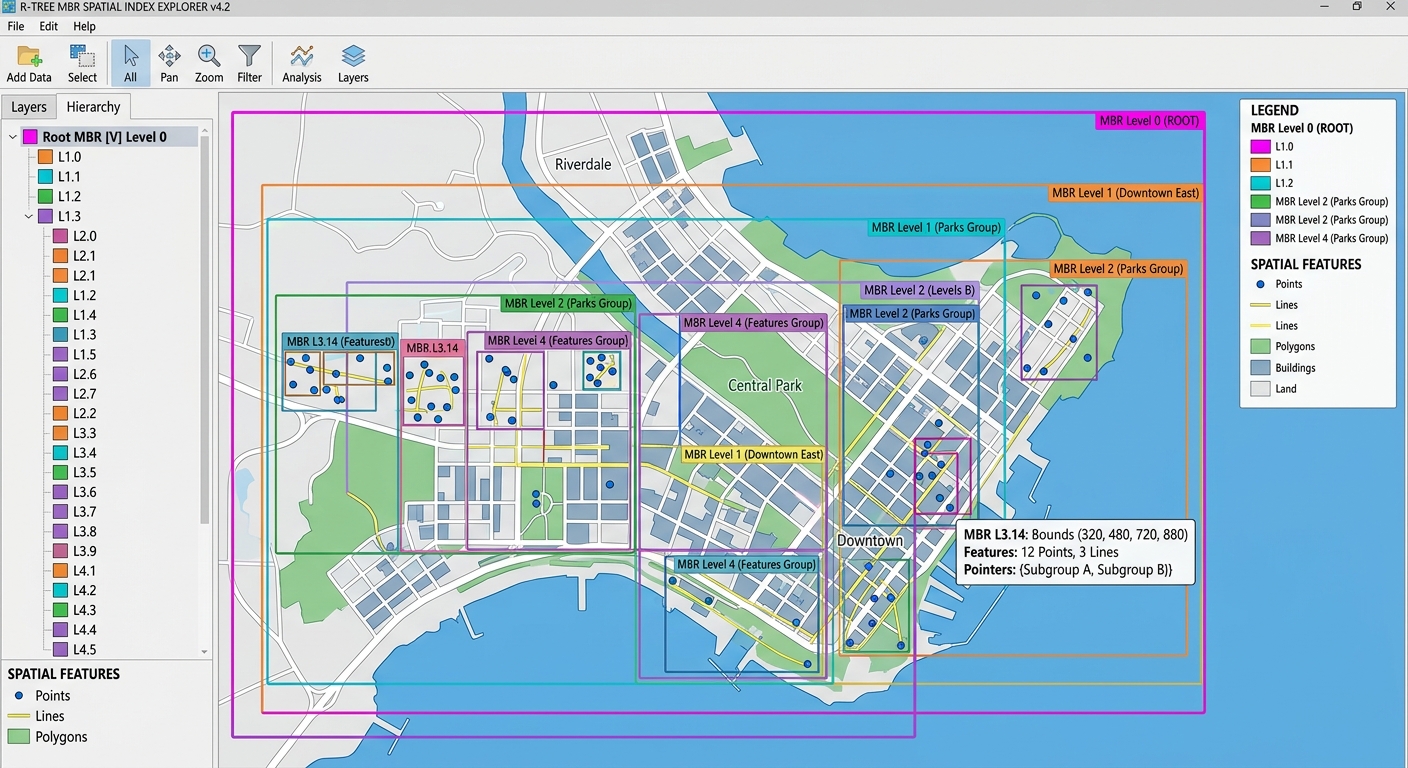
Spatial Indexing Demystified: R-Trees and B-Trees in PostGIS
1. Introduction: Why Spatial Indexing Matters
Understanding Spatial Indexing in PostGIS is critical when managing large geospatial datasets like millions of buildings and road networks. Imagine managing a PostGIS database containing five million buildings, road segments, land parcels, and utility networks. A city planner asks a seemingly simple question: Which buildings intersect a proposed road corridor?
Without a suitable spatial index, PostgreSQL may need to examine a large proportion of the building records and evaluate their geometries against the corridor. On a large dataset, this can lead to expensive queries and slow GIS applications.
Spatial indexing solves this problem by organizing geographical information so the database can locate potential matches without testing every geometry individually.
PostgreSQL provides several index types, each designed for different kinds of searches. B-Tree indexes are excellent for ordered values such as numbers, dates, and strings. GiST (Generalized Search Tree) indexes, commonly used by PostGIS for spatial data, support efficient searches involving geometric relationships.
For example, an attribute query can use a B-Tree:
SELECT *
FROM buildings
WHERE building_id = 1250;
A spatial query can use a GiST index on the geometry column:
SELECT building_id
FROM buildings
WHERE ST_Intersects(
    geom,
    ST_MakeEnvelope(
        500000, 4500000,
        501000, 4501000,
        26918
    )
);
The envelope defines a rectangular search region in the example’s projected coordinate system, EPSG:26918. Your coordinates and SRID must match your actual study area.
With a suitable spatial index, PostgreSQL can narrow the search to likely candidates before performing the exact intersection test. Depending on the dataset and query, this can reduce execution time dramatically, sometimes from minutes to milliseconds.
However, an index does not guarantee a particular speedup. The benefit depends on the dataset size, geometry complexity, search area, hardware, and execution plan.
This guide explains B-Tree indexing, R-Tree-like spatial indexing through GiST, and how to benchmark and optimize PostGIS queries.
2. How B-Tree Indexing Works
2.1 Understanding the B-Tree Structure
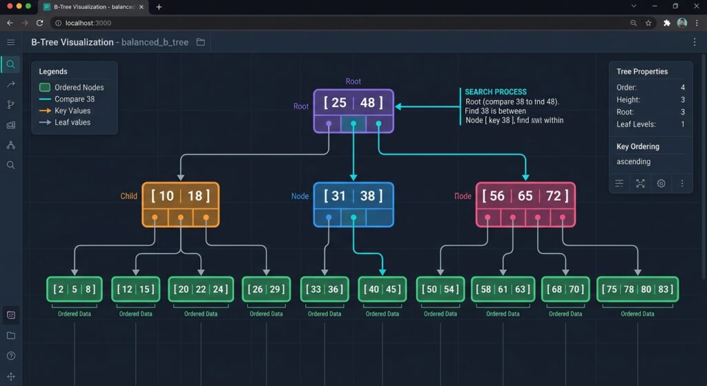
A B-Tree is a balanced search-tree structure that organizes values in an ordered manner.
Think of a library catalog organized alphabetically. Instead of opening every book to find a title, the catalog allows you to narrow the search by following an ordered structure.
A conceptual representation looks like this:
                 [50]
                /    \
          [20, 35]   [70, 90]
           /  |  \    /  |  \
          ... ... ... ... ... ...

             Ordered values
This diagram illustrates the concept rather than PostgreSQL’s exact internal page structure.
PostgreSQL B-Tree indexes are suitable for equality and range conditions, including =, <, >, BETWEEN, and many ORDER BY operations. They are commonly used with numeric, date, and text columns.
Reference: PostgreSQL B-Tree documentation.
2.2 Practical Example: Searching Attributes
Suppose a building inventory contains the following fields:
| building_id | building_type | floors | assessed_value |
|---|---|---|---|
| 101 | Residential | 2 | 4,500,000 |
| 102 | Commercial | 5 | 18,000,000 |
| 103 | Residential | 1 | 2,800,000 |
| 104 | Industrial | 3 | 12,000,000 |
You want to identify properties within a particular valuation range.
Create a B-Tree index:
CREATE INDEX idx_buildings_value
ON buildings (assessed_value);
Then run:
SELECT building_id, assessed_value
FROM buildings
WHERE assessed_value BETWEEN 4000000 AND 15000000;
The database can use the ordered index to locate potentially matching values without necessarily scanning the entire table.
B-Tree indexes are also useful for other attribute-based searches:
CREATE INDEX idx_buildings_type
ON buildings (building_type);
SELECT *
FROM buildings
WHERE building_type = 'Residential';2.3 Why B-Trees Are Not the Right Default for Spatial Queries
A geometry is not simply a number or string with a natural linear ordering. A polygon has an extent, a line follows a path, and a point occupies a position in space.
A query such as WHERE assessed_value > 10000000 benefits from an index that organizes values along an ordered dimension.
A query such as WHERE ST_Intersects(geom, search_area) instead asks about a geometric relationship involving two or more spatial dimensions.
A conventional B-Tree does not provide the spatial search structure needed for efficient general-purpose geometry intersection queries.
This does not mean B-Trees are unsuitable for GIS databases. They remain valuable for filtering spatial records by attributes, such as parcel IDs, dates, and administrative codes. The key is to select an index appropriate to the operation being performed.
PostgreSQL supports several index methods, including B-Tree, GiST, SP-GiST, and BRIN. See the PostgreSQL index types reference.
3. How R-Tree Spatial Indexing Works in PostGIS
3.1 What Is an R-Tree?
An R-Tree is a spatial indexing structure that organizes objects using hierarchical rectangular bounding regions.
A minimum bounding rectangle (MBR) is the smallest axis-aligned rectangle that completely contains a geometry in the indexed dimensions.
For example, an irregular parcel polygon may contain dozens of vertices. Its two-dimensional bounding rectangle can be represented using four values:
- Minimum X coordinate
- Minimum Y coordinate
- Maximum X coordinate
- Maximum Y coordinate
Testing whether two rectangles overlap is generally less expensive than performing a detailed geometric comparison between complex polygons.
A conceptual hierarchy looks like this:
                ROOT BOUNDING BOX
               /                  \
        WESTERN REGION          EASTERN REGION
          /       \               /       \
      BOX A       BOX B         BOX C     BOX D
        |           |             |         |
     Features    Features      Features  Features
The index uses bounding regions to narrow the search to promising areas of the tree. It does not need to examine every feature’s full geometry during the initial search.
3.2 GiST Versus R-Tree: Understanding the Terminology
These terms describe related but different concepts.
GiST stands for Generalized Search Tree. It is a PostgreSQL index framework that supports different searchable data structures through appropriate operator classes.
R-Tree describes a family of spatial index structures based on hierarchical bounding regions.
PostGIS commonly implements R-Tree-like spatial indexing using the GiST access method. This is why the standard index definition for a PostGIS geometry column uses USING GIST.
CREATE INDEX idx_buildings_geom
ON buildings
USING GIST (geom);
The statement creates a GiST index on the geometry column named geom.
For the default PostGIS geometry operator class, the index is two-dimensional. Specialized n-dimensional operator classes are available for workloads requiring different spatial dimensions.
See the PostGIS spatial index documentation.
3.3 How Bounding Box Spatial Searches Work
Suppose an analyst wants every building intersecting a proposed construction site.
The database can approach the query in two stages.
Stage 1: Bounding box filtering
The index identifies geometries whose bounding boxes overlap the search region’s bounding box.
Stage 2: Exact geometry testing
PostGIS evaluates the actual spatial predicate on the candidate geometries to determine which records satisfy the requested relationship.
This is important because bounding box overlap does not necessarily mean that two geometries intersect. An irregular polygon may have a bounding rectangle containing large empty areas.
For example:
SELECT building_id
FROM buildings
WHERE ST_Intersects(
    geom,
    ST_MakeEnvelope(
        500000, 4500000,
        501000, 4501000,
        26918
    )
);
ST_Intersects is an index-aware PostGIS function. When the query planner determines that using the spatial index is cost-effective, it can use the index to filter candidate features before performing the exact spatial test.
This combination of coarse filtering and exact testing is one of the main reasons PostGIS can efficiently handle large spatial datasets.
Reference: PostGIS spatial query documentation.
4. Step-by-Step PostGIS Implementation: Testing Spatial Index Performance
The most reliable way to understand spatial indexing is to benchmark the same query before and after creating an index.
This example assumes a table named buildings containing a unique identifier, building_id, and a PostGIS geometry column, geom.
Step 1: Verify the Table and Geometry
First, confirm that PostGIS is available:
CREATE EXTENSION IF NOT EXISTS postgis;This statement requires the appropriate database permissions and does not need to be repeated when the extension is already enabled.
Check the table structure:
SELECT
    column_name,
    data_type
FROM information_schema.columns
WHERE table_name = 'buildings';
Inspect the geometry type and SRID:
SELECT
    GeometryType(geom) AS geometry_type,
    ST_SRID(geom) AS srid,
    COUNT(*) AS feature_count
FROM buildings
WHERE geom IS NOT NULL
GROUP BY GeometryType(geom), ST_SRID(geom);
Ensure that the search geometry uses a compatible coordinate reference system. For projected geometries, the envelope coordinates are typically expressed in the CRS’s linear units.
Step 2: Execute the Query Without a Spatial Index
For a clean comparison, conduct the benchmark in a test database or on a dedicated test copy of the table.
Do not remove a production index solely to run an experiment. If an existing spatial index is present, inspect it first and use an isolated test environment for the no-index measurement.
In the test environment, remove the relevant index if necessary:
DROP INDEX IF EXISTS idx_buildings_geom;Now execute the spatial query with EXPLAIN ANALYZE:
EXPLAIN (ANALYZE, BUFFERS)
SELECT building_id
FROM buildings
WHERE ST_Intersects(
    geom,
    ST_MakeEnvelope(
        500000, 4500000,
        501000, 4501000,
        26918
    )
);
EXPLAIN ANALYZE executes the query and reports actual timing, row counts, and execution-plan details. The BUFFERS option reports information about the data pages accessed.
Without a usable spatial index, a typical plan on a sufficiently large table might contain a sequential scan:
Seq Scan on buildings
  Filter: st_intersects(geom, ...)
  Rows Removed by Filter: ...
Planning Time: ...
Execution Time: ...
The database examines table records and evaluates the spatial filter against them.
A sequential scan is not automatically inefficient. It can be the correct plan for a small table or a query that matches a large proportion of the dataset.
Record the actual execution time and buffer statistics from your own database. The output above illustrates the plan shape rather than representing a measured benchmark.
Step 3: Create a GiST Spatial Index
Create the spatial index:
CREATE INDEX idx_buildings_geom
ON buildings
USING GIST (geom);
This command builds a GiST index on the geometry column. For spatial searches, it allows PostgreSQL to locate candidate geometries based on their indexed bounding regions.
For a large production table that must remain available for normal writes, you may instead use concurrent index creation:
CREATE INDEX CONCURRENTLY idx_buildings_geom
ON buildings
USING GIST (geom);
Use one command or the other, not both in succession.
CREATE INDEX CONCURRENTLY reduces write blocking during index creation but has additional overhead and cannot run inside a transaction block. Plan index creation around available storage, workload, and operational requirements.
Step 4: Refresh the Table Statistics
After a large data load or major change to the table, refresh statistics if necessary:
ANALYZE buildings;Alternatively, run routine maintenance and analysis together:
VACUUM ANALYZE buildings;ANALYZE collects statistics that help the query planner estimate the number of matching records and choose an efficient execution plan.
VACUUM helps reclaim space occupied by obsolete row versions so that the space can be reused.
PostgreSQL’s autovacuum and autoanalyze processes may already maintain the table adequately. Manual commands should be guided by the workload and maintenance requirements.
See the PostgreSQL VACUUM reference and ANALYZE reference.
Step 5: Re-run the Identical Query
Use the same query and search extent as before:
EXPLAIN (ANALYZE, BUFFERS)
SELECT building_id
FROM buildings
WHERE ST_Intersects(
    geom,
    ST_MakeEnvelope(
        500000, 4500000,
        501000, 4501000,
        26918
    )
);
A selective query may now produce a plan like this:
Bitmap Heap Scan on buildings
  Recheck Cond: (geom && ...)
  Filter: st_intersects(geom, ...)
  -> Bitmap Index Scan on idx_buildings_geom
       Index Cond: (geom && ...)
Planning Time: ...
Execution Time: ...
Alternatively, PostgreSQL may use an Index Scan.
The bounding box condition identifies candidate geometries, and the exact intersection predicate checks them. Some candidates may fail the final test, which is normal.
The planner can still choose a sequential scan if the table is small, the search covers much of the dataset, or index access is estimated to be more expensive.
Step 6: Compare Before-and-After Performance
Record the measured outputs in a table:
| Metric | Without spatial index | With GiST index |
|---|---|---|
| Execution plan | Often sequential scan | Index scan or bitmap-assisted scan when cost-effective |
| Records examined | Potentially many table records | Often fewer candidate records for selective searches |
| Exact geometry tests | May evaluate many geometries | Usually restricted to potential matches |
| Execution time | Record measured result | Record measured result |
| Buffer activity | Record measured result | Record measured result |
You can calculate the speedup using:
[
\text{Speedup}=
\frac{\text{Execution time without index}}
{\text{Execution time with index}}
]
For example, suppose a test query takes 12 seconds without the spatial index and 0.4 seconds with it. The measured speedup would be:
[
\text{Speedup}=\frac{12}{0.4}=30
]
These times are hypothetical and are not claimed as results from an actual database benchmark.
For a more reliable test, repeat the query, keep its parameters identical, distinguish warm-cache performance from cold-cache behavior where relevant, and inspect both execution time and buffer activity.
The objective is to measure the index’s effect on your workload rather than assume that every spatial query will become faster.
5. Best Practices for Accelerating Spatial Queries in PostgreSQL
5.1 Use Index-Aware Spatial Predicates
PostGIS includes several spatial predicates and functions that can use spatial indexes to reduce the number of candidate geometries.
Common examples include:
ST_IntersectsST_ContainsST_WithinST_CoversST_OverlapsST_DWithin
For example, to find buildings within 500 metres of a transit station:
SELECT b.building_id
FROM buildings AS b
JOIN transit_stations AS s
    ON ST_DWithin(b.geom, s.geom, 500)
WHERE s.station_id = 25;
The distance value uses the units of the geometry’s projected CRS. If the geometry uses longitude and latitude, choose an appropriate geography or distance-based approach instead of assuming the units are metres.
ST_DWithin is index-aware and can accelerate proximity queries when the data, predicate, and execution plan are suitable.
5.2 Understand the Bounding Box Operator
The && operator tests whether the two-dimensional bounding boxes of two geometries overlap or touch.
For example:
SELECT building_id
FROM buildings
WHERE geom && ST_MakeEnvelope(
    500000, 4500000,
    501000, 4501000,
    26918
);
This query returns features based on bounding box overlap. It does not guarantee that the actual geometries intersect.
Use && when approximate bounding box filtering is what you need. Use ST_Intersects or another suitable predicate when you require the exact geometric relationship.
5.3 Avoid Unnecessary Transformations on Indexed Geometry
Applying a transformation directly to an indexed column can prevent the ordinary index on that column from being used as expected.
For example:
-- May prevent use of the ordinary index on geom
SELECT building_id
FROM buildings
WHERE ST_Intersects(
    ST_Transform(geom, 4326),
    ST_SetSRID(
        ST_MakeEnvelope(
            -73.99, 40.70,
            -73.98, 40.71
        ),
        4326
    )
);
When possible, transform the search geometry into the CRS of the indexed column instead:
SELECT building_id
FROM buildings
WHERE ST_Intersects(
    geom,
    ST_Transform(
        ST_SetSRID(
            ST_MakeEnvelope(
                -73.99, 40.70,
                -73.98, 40.71
            ),
            4326
        ),
        26918
    )
);
This example assumes that EPSG:26918 is appropriate for the stored geometries and the search location.
The general principle is to preserve the indexed column in its indexed form whenever practical, while ensuring that the spatial reference systems are valid and compatible.
5.4 Maintain Statistics After Major Data Changes
After bulk loading, large deletions, or substantial updates, check whether the planner’s statistics are current.
ANALYZE buildings;For routine maintenance where both operations are appropriate:
VACUUM ANALYZE buildings;VACUUM ANALYZE is useful for maintaining table health and updating planner statistics. It is not a magic command that guarantees a faster query, and an index does not need to be rebuilt every time the table changes.
Avoid treating VACUUM FULL as routine maintenance. It rewrites the table and requires an exclusive lock, so it can be disruptive on production systems.
5.5 Manage Indexes in Enterprise Databases
Spatial indexes consume storage and add work to inserts, updates, and deletes. Create them where they provide measurable benefits.
For example:
CREATE INDEX idx_parcels_geom
ON parcels
USING GIST (geom);

CREATE INDEX idx_roads_geom
ON roads
USING GIST (geom);
Maintain descriptive index names and monitor important query plans over time.
If a query remains slow despite an existing spatial index, investigate:
- Whether the execution plan actually uses the index.
- Whether the search region is too large to benefit from index filtering.
- Whether table statistics are current.
- Whether the indexed geometries have unusually large bounding boxes.
- Whether expensive exact geometry calculations or large result sets dominate the runtime.
- Whether transformations or other expressions prevent expected index usage.
For very large tables, other index methods may also be relevant. PostGIS supports BRIN indexes for some data whose physical storage order correlates with spatial location, and SP-GiST for supported partitioned search structures. GiST remains a widely used general-purpose option for spatial geometry.
5.6 Be Careful with Three-Dimensional Data
The default PostGIS GiST geometry index is two-dimensional. Geometries can store Z coordinates, but the existence of Z values does not automatically make an ordinary two-dimensional spatial predicate perform three-dimensional filtering.
For a workload that requires n-dimensional indexing, PostGIS supports a specialized operator class:
CREATE INDEX idx_assets_geom_nd
ON assets
USING GIST (geom gist_geometry_ops_nd);
Use this only when the data and query operators require n-dimensional indexing. Make sure the predicates used by the workload are compatible with the chosen operator class.
6. Summary Comparison: B-Trees and R-Tree-Like GiST Indexes
| Feature | B-Tree index | R-Tree-like GiST spatial index |
|---|---|---|
| Primary purpose | Ordered attribute searches | Spatial candidate filtering |
| Structure | Balanced hierarchy of ordered values | Hierarchical bounding regions |
| Suitable columns | Integers, prices, dates, strings | Points, lines, polygons, and other supported geometries |
| Example search | WHERE age > 30 |
WHERE ST_Intersects(geom, area) |
| Spatial relationships | Not the general-purpose choice | Designed to accelerate supported spatial predicates |
| Exact geometry testing | Not its main role | Narrows candidates; exact predicates verify matches |
| PostgreSQL syntax | CREATE INDEX ... ON table(column) |
CREATE INDEX ... ON table USING GIST(geom) |
| Main trade-off | Storage and write overhead | Storage, index maintenance, and write overhead |
7. Conclusion
Spatial indexing is fundamental to efficient PostGIS database design.
B-Tree indexes help PostgreSQL efficiently search ordered attributes, while GiST-based spatial indexes use hierarchical bounding regions to identify candidate geometries for supported spatial queries.
The practical workflow is straightforward: benchmark a representative query with EXPLAIN ANALYZE, create the appropriate GiST index, refresh statistics when necessary, and measure the same query again.
For production systems, index design should be based on actual query patterns, execution plans, storage constraints, and maintenance requirements.
The central lesson: Choose the right index for the operation, use index-aware spatial predicates, and verify performance empirically. A spatial index can dramatically accelerate selective GIS queries, but sound query design and ongoing database maintenance remain essential.
References
- PostGIS: Spatial indexes — GiST indexing, bounding boxes, and index-aware functions.
- PostGIS: Spatial queries — spatial predicates and index-assisted filtering.
- PostgreSQL: B-Tree indexes — ordered attribute searching.
- PostgreSQL: EXPLAIN — execution plans and performance measurement.
- PostgreSQL: VACUUM — table maintenance and
VACUUM ANALYZE.