Table of Contents

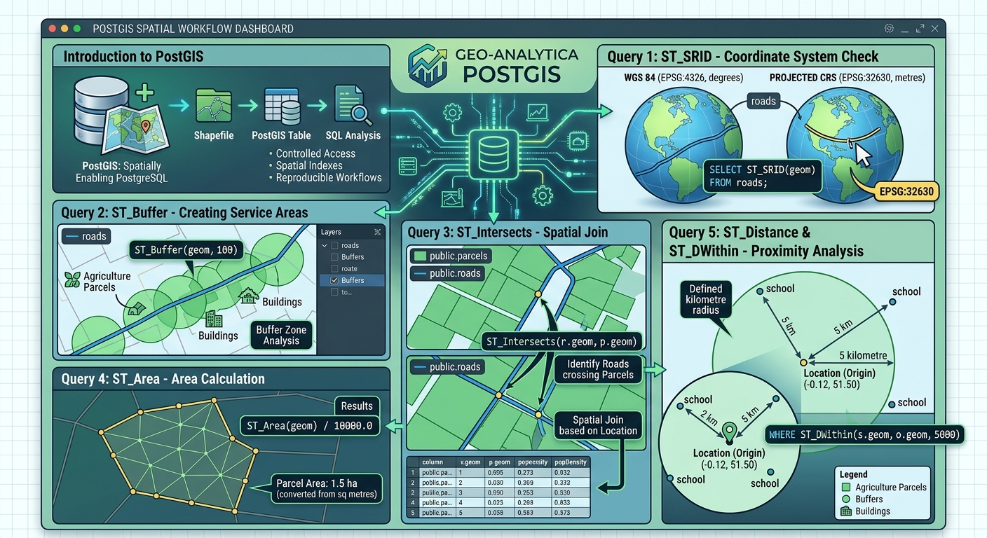
PostGIS Starter Guide: 5 Spatial SQL Queries Every GIS Student Should Know

1. Introduction: Why GIS Students Should Learn PostGIS

Welcome to this comprehensive PostGIS Starter Guide spatial SQL queries overview, designed to help GIS students master database management. Traditional GIS workflows often rely on individual files such as Shapefiles, GeoJSON, and GeoPackage datasets. These formats are valuable for mapping and data exchange, but managing many files can become difficult when projects involve large datasets, multiple analysts, frequent updates, or complex spatial relationships.

PostGIS extends PostgreSQL, a relational database management system, with spatial data types, spatial functions, and spatial indexing. It allows GIS professionals to store geographic features in database tables and analyse them using Structured Query Language (SQL).

Instead of manually selecting roads within a particular distance of schools, for example, you can write one spatial SQL query that finds the relevant features and returns their distances.

Why move from Shapefiles to PostgreSQL and PostGIS?

File-based GIS	PostgreSQL + PostGIS
Data commonly managed as separate files	Spatial and attribute data managed in database tables
Complex analysis often performed through desktop tools	Spatial analysis can be executed directly in SQL
Concurrent editing and access can be difficult to coordinate	Supports controlled access for multiple users
Large spatial searches may require repeated processing	Spatial indexes can accelerate suitable queries
Workflows often depend on desktop processing steps	Queries can be saved, reused, documented, and automated

PostGIS is particularly useful for urban planning, environmental management, transportation, cadastral mapping, remote sensing, and web GIS development.

This beginner guide introduces five essential spatial SQL queries that GIS students can use in academic assignments and professional projects.

2. Setting Up PostgreSQL and PostGIS

Before running spatial queries, you need a PostgreSQL database with the PostGIS extension enabled. Using a reliable **PostGIS Starter Guide spatial SQL queries** workflow ensures your database environment is properly configured.

Step 1: Install the required software

Install PostgreSQL and a compatible PostGIS version using the official PostGIS installation documentation.

You can use either pgAdmin, a graphical administration tool for PostgreSQL, or QGIS DB Manager to connect to your database and execute SQL.

Step 2: Create a database and enable PostGIS

Create a database for your GIS project, for example, gis_student_db.

Open the SQL query interface for that database and execute:

-- Enable spatial functionality in this database.
CREATE EXTENSION IF NOT EXISTS postgis;

-- Check the installed PostGIS version.
SELECT PostGIS_Full_Version();

The first statement enables PostGIS spatial types and functions. The second returns information about the installed PostGIS version and its build configuration.

Your database administrator account must have permission to install the extension.

Step 3: Connect through QGIS DB Manager

In QGIS:

Open Database → DB Manager → DB Manager.
Expand the PostgreSQL section and select your connection, or create a new connection.
Enter your server host, port, database name, username, and password.
Connect to the database.
Select the database and open the SQL window to execute queries.

For a local installation, the host is commonly localhost and the default PostgreSQL port is 5432, unless your configuration specifies otherwise.

QGIS DB Manager can also import GIS files into PostGIS tables and inspect their geometry information. See the QGIS DB Manager documentation.

Step 4: Connect through pgAdmin

Alternatively, open pgAdmin and connect to your PostgreSQL server. Expand Servers → your server → Databases → gis_student_db, then right-click the database and select Query Tool.

Enter your SQL statements in the query editor and execute them using the interface’s Run command.

Step 5: Prepare example GIS tables

For the queries below, assume your database contains these tables:

Table	Geometry type	Example attributes	Purpose
`public.roads`	LineString	`id`, `road_name`, `geom`	Road network
`public.parcels`	Polygon	`id`, `parcel_name`, `geom`	Land parcels
`public.schools`	Point	`id`, `school_name`, `geom`	School locations

Here, geom is the geometry column.

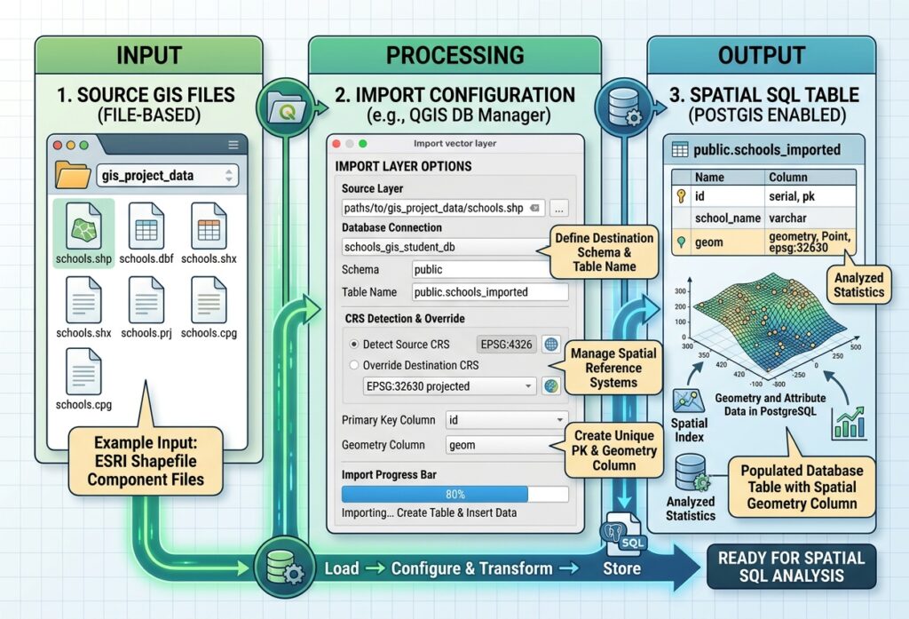
Import your own layers using QGIS DB Manager → Import Layer/File, or another supported import method. The queries assume that the tables are in the public schema and use the field names shown above. Replace these names with the corresponding names in your own database.

For metric examples, we will use EPSG:32630 as an illustrative projected coordinate system for a study area near London. Replace it with an appropriate projected CRS for your actual study area. The sample tables used for the metric queries should already have been transformed to that CRS, with coordinates expressed in metres.

3. Query 1: Importing Data and Checking Spatial Reference Systems with ST_SRID

Why this query matters

Every spatial dataset has a coordinate reference system (CRS), either explicitly defined or missing. Before combining layers or measuring distances, you need to understand how their coordinates are represented.

The PostGIS function ST_SRID() returns the Spatial Reference System Identifier (SRID) associated with a geometry.

An SRID such as 4326 identifies WGS 84 geographic coordinates, commonly represented as longitude and latitude. A projected CRS such as EPSG:32630 represents coordinates in a projected grid, measured in metres.

Step 1: Import a GIS layer

In QGIS DB Manager:

Connect to your PostGIS database.
Choose Table → Import Layer/File.
Select the vector layer you want to import.
Enter the destination schema and table name.
Check the layer’s geometry and CRS information.
Run the import and confirm the table appears in the database.

A successful import creates a database table containing the feature attributes and a geometry column.

Step 2: Inspect the spatial reference system

Run this query:

-- Check the SRID and geometry type of imported roads.
SELECT
    id,
    ST_SRID(geom) AS srid,
    GeometryType(geom) AS geometry_type
FROM public.roads
LIMIT 10;

Expected output:

id	srid	geometry_type
1	32630	LINESTRING
2	32630	LINESTRING
3	32630	LINESTRING

The displayed values are illustrative. Your actual SRID and geometry types depend on the imported dataset.

You can also inspect the CRS registered for your database layers:

-- List known spatial tables and their geometry metadata.
SELECT
    f_table_schema,
    f_table_name,
    f_geometry_column,
    type,
    srid
FROM geometry_columns
WHERE f_table_schema = 'public'
ORDER BY f_table_name;

This query lists spatial tables recognised by PostGIS and reports their geometry column, type, and SRID.

Important distinction: ST_SetSRID versus ST_Transform

These two functions solve different problems.

ST_SetSRID(geom, 4326) assigns CRS metadata to a geometry. It does not change the coordinate values.
ST_Transform(geom, 32630) converts the coordinates into the target CRS.

For example, if a dataset’s coordinates are genuinely longitude and latitude in WGS 84, transforming them to a suitable projected CRS changes their numeric coordinates to the corresponding projected values.

Do not use ST_SetSRID() simply to make an incorrectly labelled layer appear to match another layer. First determine the CRS in which the coordinates are actually expressed.

When to use it: Before spatial joins, distance calculations, buffer analysis, or combining datasets from different sources.

4. Query 2: Creating Vector Buffers with ST_Buffer

A buffer is a polygon representing an area within a specified distance of a geographic feature.

For example, a 100-metre buffer around a road can help identify nearby buildings, agricultural parcels, or other features potentially affected by road access or roadside activities. When following a **PostGIS Starter Guide spatial SQL queries** approach for buffers, spatial automation becomes straightforward.

The PostGIS function ST_Buffer() creates the buffer geometry.

SQL query: Buffer all roads by 100 metres

Assuming public.roads.geom uses a suitable projected CRS with metre units:

-- Create a 100-metre buffer around each road.
SELECT
    id,
    road_name,
    ST_Buffer(geom, 100) AS buffer_geom
FROM public.roads;

What does the query do?

Reads each feature in the roads table.
Uses the road geometry as the input.
Generates a buffer extending 100 metres around the line.
Returns the buffer geometry alongside the road attributes.

For a line feature, the result is generally a polygon surrounding the road. The output is a query result until you explicitly save it to a table or export it.

Save the buffers as a new database table

To create a reusable output table, run:

-- Create a table of road buffers in the projected CRS.
CREATE TABLE public.road_buffers_100m AS
SELECT
    id AS road_id,
    road_name,
    ST_Buffer(geom, 100) AS geom
FROM public.roads;

This creates public.road_buffers_100m with a geometry column containing the buffer polygons.

The query will fail if that table already exists. For repeated workflows, either remove the previous output intentionally or choose a new table name.

What if your data uses longitude and latitude?

A buffer distance must be expressed in meaningful units. If the source geometry uses EPSG:4326, its coordinate units are angular degrees rather than metres.

For a suitable local projected CRS, you can transform the geometry before buffering:

-- Example only: replace 32630 with your local metric CRS.
SELECT
    id,
    ST_Buffer(ST_Transform(geom, 32630), 100) AS buffer_geom
FROM public.roads;

The buffer in this example is 100 metres because the target CRS uses metres.

When to use it: Road-access studies, service areas, environmental impact zones, proximity analysis, and preliminary planning buffers.

5. Query 3: Spatial Joins and Intersections with ST_Intersects

Traditional SQL joins usually match records through shared attribute values, such as an ID or category. A spatial join matches features according to their geographic relationships.

PostGIS provides several spatial predicates for these operations. One of the most widely used is ST_Intersects().

It returns TRUE when two geometries share at least one point in space. Their interiors do not necessarily have to overlap: lines crossing, polygons overlapping, and geometries touching at a boundary can all satisfy the predicate.

SQL query: Find roads that intersect parcels

-- Match roads to every parcel they intersect.
SELECT
    r.id AS road_id,
    r.road_name,
    p.id AS parcel_id,
    p.parcel_name
FROM public.roads AS r
JOIN public.parcels AS p
    ON ST_Intersects(r.geom, p.geom);

What does the query do?

The database compares road and parcel geometries. Whenever a road and a parcel intersect, the query returns a record containing the IDs and attributes of both features.

A road that crosses five parcel polygons may appear in five rows. This is expected because one road can have a spatial relationship with multiple parcels.

The input layers must use compatible coordinate systems. The example assumes that the geometry values are expressed in the same CRS.

Clip intersecting roads to parcel boundaries

Sometimes, knowing that two features intersect is not enough. You may want to obtain the exact part of a road that lies within a parcel.

Use ST_Intersection(), which calculates the geometry shared by its inputs.

-- Return the section of each road lying inside or on a parcel.
SELECT
    r.id AS road_id,
    p.id AS parcel_id,
    ST_Intersection(r.geom, p.geom) AS intersection_geom
FROM public.roads AS r
JOIN public.parcels AS p
    ON ST_Intersects(r.geom, p.geom);

The output geometry contains the intersection between each road and parcel. Depending on the features, it may be a line, point, or another geometry type.

ST_Intersects() is a spatial predicate used to test a relationship; ST_Intersection() is a geometry operation that constructs the shared geometry. Understanding this difference is essential when writing spatial SQL.

When to use it: Overlay analysis, land administration, road-network studies, identifying facilities within administrative areas, and linking satellite-derived features to management zones.

6. Query 4: Calculating Lengths and Areas with ST_Length and ST_Area

GIS projects often require measurements such as road length, river length, parcel area, forest extent, or the area of a floodplain.

PostGIS provides two essential functions:

ST_Length() calculates the length of a line geometry.
ST_Area() calculates the area of a polygon geometry.

For geometry-based calculations, the returned units follow the geometry’s CRS units. A projected CRS using metres gives line lengths in metres and polygon areas in square metres.

SQL query A: Calculate road lengths

-- Calculate the length of each road in metres.
SELECT
    id,
    road_name,
    ST_Length(geom) AS length_m
FROM public.roads
ORDER BY length_m DESC;

The result contains each road’s stored geometry length, ordered from longest to shortest.

If road geometries are segmented, the query measures each stored feature. It does not automatically combine road segments sharing the same name.

SQL query B: Calculate parcel areas

-- Calculate the area of each parcel in square metres.
SELECT
    id,
    parcel_name,
    ST_Area(geom) AS area_m2
FROM public.parcels
ORDER BY area_m2 DESC;

This query returns the area of every parcel polygon based on its geometry.

Convert area to hectares

One hectare equals 10,000 square metres, so you can convert the calculated area directly:

-- Calculate parcel area in hectares.
SELECT
    id,
    parcel_name,
    ST_Area(geom) / 10000.0 AS area_ha
FROM public.parcels;

The decimal divisor avoids integer-style division concerns and keeps the result suitable for reporting.

Important: These queries assume the road and parcel geometry columns are stored in a projected CRS with metre units. If the source is in longitude and latitude, do not calculate planar lengths or areas directly from those degree coordinates. Transform the geometry to a suitable local projected CRS first, or use geography-based calculations when appropriate.

For example, for a table whose geometries are in WGS 84:

-- Example projected calculation; choose the correct CRS for your area.
SELECT
    id,
    ST_Area(ST_Transform(geom, 32630)) AS area_m2
FROM public.parcels;

The CRS in this example is illustrative and should be replaced with the appropriate projected CRS for the study area.

These functions calculate measurements from the geometry as stored. Their real-world accuracy also depends on the quality, scale, completeness, and validity of the source data.

When to use it: Cadastral mapping, land-cover assessment, road inventory, watershed analysis, environmental reporting, and agricultural field measurement.

7. Query 5: Finding Nearby Features with ST_DWithin and ST_Distance

Nearest-neighbour analysis is useful when answering questions such as:

Which school is closest to a particular settlement?
Which clinic lies within five kilometres of a village?
Which road is nearest to an agricultural field?
Which monitoring station is closest to a river reach?

Two important functions are ST_DWithin() and ST_Distance().

ST_DWithin() tests whether two geometries fall within a specified distance. ST_Distance() calculates the distance between them.

SQL query: Find schools within five kilometres of a location

Assume the schools.geom column uses the projected CRS EPSG:32630. The following example uses a sample location near London, expressed initially in longitude and latitude.

-- Define an example origin and find schools within 5 km.
WITH origin AS (
    SELECT ST_Transform(
        ST_SetSRID(
            ST_MakePoint(-0.12, 51.50),
            4326
        ),
        32630
    ) AS geom
)
SELECT
    s.id,
    s.school_name,
    ST_Distance(s.geom, o.geom) AS distance_m
FROM public.schools AS s
CROSS JOIN origin AS o
WHERE ST_DWithin(s.geom, o.geom, 5000)
ORDER BY ST_Distance(s.geom, o.geom)
LIMIT 5;

How the query works:

ST_MakePoint() creates a point from the example longitude and latitude.
ST_SetSRID(..., 4326) identifies the point’s coordinate reference system as WGS 84.
ST_Transform(..., 32630) transforms the point to the projected CRS used by the schools table.
ST_DWithin(..., 5000) filters schools within five kilometres of the origin.
ST_Distance() calculates the distance for each qualifying school.
ORDER BY ... ASC sorts the nearest schools first.
LIMIT 5 returns up to five records.

The output reports distance in metres because the example projected CRS uses metre units.

Adapt this query to your study area: Replace the sample point coordinates and use the correct source SRID and local projected CRS. Ensure your schools are actually stored in the projected CRS selected in the query.

If no schools lie within five kilometres, the query returns no rows. Increase the search radius when a broader search is appropriate.

Why use ST_DWithin instead of only ST_Distance?

A tempting approach is to filter records with a condition such as:

-- Avoid relying on this alone for large spatial tables.
WHERE ST_Distance(s.geom, o.geom) < 5000

That condition may require distance calculations for a large number of rows. By contrast, ST_DWithin() is spatial-index-aware and can use a suitable spatial index to narrow down candidate features before checking their actual distances.

The ORDER BY ST_Distance() expression then sorts the remaining candidates by distance. For large tables, this combination is a useful pattern.

PostGIS explains this behaviour in its spatial query documentation.

When to use it: Facility accessibility, nearest-road analysis, emergency planning, service-area studies, and location-based GIS applications.

8. Bonus: Improving Spatial Query Performance with Indexes

The five queries above become particularly powerful when applied to large datasets. However, spatial queries can become slow if PostgreSQL must evaluate every geometry in a table.

A spatial index helps the database identify candidate features efficiently.

PostGIS commonly uses a GiST index on a geometry column. Its geometry indexing uses an R-tree-style approach to accelerate supported spatial searches.

Create a spatial index

For example, create an index for the roads geometry:

-- Create a spatial index for the roads table.
CREATE INDEX roads_geom_gix
ON public.roads
USING GIST (geom);

-- Update table statistics for query planning.
ANALYZE public.roads;

Repeat the process for other spatial tables where suitable:

-- Create spatial indexes for parcels and schools.
CREATE INDEX parcels_geom_gix
ON public.parcels
USING GIST (geom);

CREATE INDEX schools_geom_gix
ON public.schools
USING GIST (geom);

ANALYZE public.parcels;
ANALYZE public.schools;

If a spatial index already exists, you do not need to create a duplicate.

A GiST spatial index generally indexes geometry bounding boxes. PostGIS uses those boxes to narrow the candidates, then applies the relevant spatial predicate to test the actual geometries.

For large datasets, functions such as ST_Intersects() and ST_DWithin() can benefit from this approach. See the official PostGIS spatial index guide.

Remember that an index will not guarantee faster performance for every query. The query structure, table size, data distribution, statistics, and database configuration all matter.

9. Conclusion: Building Your Spatial SQL Skills

PostGIS lets GIS professionals move beyond desktop-only processing and perform spatial analysis directly inside a relational database. Mastering the core techniques outlined in this **PostGIS Starter Guide spatial SQL queries** article prepares you for advanced geospatial roles.

The five queries in this guide provide a practical foundation:

Query	Function	Main task
1	`ST_SRID()`	Inspect coordinate reference systems
2	`ST_Buffer()`	Create distance-based buffer polygons
3	`ST_Intersects()` and `ST_Intersection()`	Find spatial relationships and construct shared geometry
4	`ST_Length()` and `ST_Area()`	Calculate line lengths and polygon areas
5	`ST_DWithin()` and `ST_Distance()`	Find nearby features and measure distances

As you progress, practise combining these functions with conventional SQL clauses such as WHERE, JOIN, GROUP BY, ORDER BY, and LIMIT.

The most important habits are to verify spatial reference systems, use suitable units for measurements, understand what each spatial predicate actually tests, and create spatial indexes where they are beneficial.

Mastering these concepts will help you build reproducible GIS workflows, manage larger spatial datasets, and prepare for professional roles involving spatial databases, web GIS, environmental analysis, and geospatial data engineering.