Table of Contents

Multi Criteria Evaluation GIS Site Selection: A Step-by-Step Site Suitability Tutorial

Introduction: What Is Multi-Criteria Evaluation in GIS?

Multi criteria evaluation GIS site selection is a spatial decision-making approach used to identify locations that best satisfy several criteria at the same time.

A typical site-selection problem might ask:

Where should a new hospital, school, warehouse, solar farm, landfill, or emergency facility be located?

The answer rarely depends on a single geographic variable. A suitable site may need to:

Be close to roads.
Have gentle slopes.
Avoid rivers and flood-prone areas.
Be located on appropriate land cover.
Remain a certain distance from settlements.
Have sufficient available land.

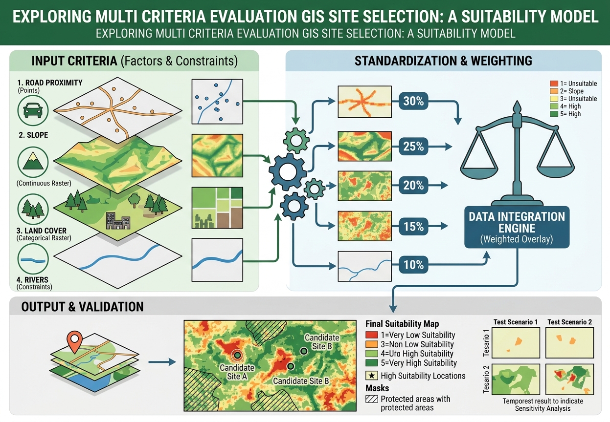
Multi-Criteria Evaluation (MCE) combines these factors into a single suitability model. A common approach is weighted overlay analysis, where each criterion is standardized to a common suitability scale and then assigned a weight according to its relative importance.

The basic concept is:

Raw spatial data → standardized suitability scores → weighted combination → suitability map → validation

This workflow is widely used in GIS planning, environmental assessment, urban planning, infrastructure development, agriculture, and renewable-energy site selection.

1. Understand the Structure of a Site Suitability Model

Before opening ArcGIS Pro or QGIS, separate your criteria into two categories:

Factors

A factor contributes positively or negatively to suitability on a continuous scale.

Examples:

Distance from roads
Slope
Distance from rivers
Distance from settlements
Elevation

Constraints

A constraint identifies areas that should not be considered at all.

Examples:

Protected areas
Existing buildings
Water bodies
Airports
Legally restricted zones
Floodways

This distinction is important.

A factor might say:

“Closer to a road is generally more suitable.”

A constraint says:

“This area cannot be used regardless of its other characteristics.”

2. Define the Decision Problem

Start by writing a precise statement of the problem.

For example:

Objective: Identify suitable locations for a new community health facility.

Then establish the geographic study area.

For example:

One municipality
A county
A watershed
An urban district
A regional planning zone

Define the study area before processing the criteria so that all datasets are analyzed over the same geographic extent.

3. Establish Your Suitability Criteria

For a simple student project, you might select:

Distance to roads
Slope
Land cover
Distance from rivers
Distance from settlements

However, the criteria should be justified by the actual planning problem.

For a hospital, road accessibility might be highly important.

For a solar farm, slope and solar-resource conditions might receive greater attention.

For a landfill, distance from settlements and environmentally sensitive areas may be critical.

Do not choose criteria simply because the datasets are available.

Every criterion should answer:

Why should this variable influence site suitability?

4. Establish Buffer Distance Constraints

Some suitability problems require minimum separation distances.

For example, you may decide that candidate sites must be:

At least 100 m from rivers.
At least 500 m from major settlements.
Within 2 km of roads.
Outside protected areas.

These distances should ideally come from:

Planning regulations
Environmental guidelines
Engineering requirements
Published literature
The project’s stated assumptions

If you are completing a university assignment and no official threshold is provided, clearly label your distances as project assumptions rather than presenting them as universal standards.

5. Prepare the Input Data

Collect the required GIS layers.

A typical project might contain:

Dataset	Geometry	Possible Use
Roads	Line	Accessibility
Rivers	Line	Environmental constraint
Settlements	Point/Polygon	Population access or exclusion
Land cover	Raster	Land-use suitability
DEM	Raster	Slope
Protected areas	Polygon	Constraint

Before analysis, inspect every dataset.

Check:

CRS
Extent
Resolution
Units
Geometry
Missing values
Attribute fields

6. Use a Common Projected CRS

Distance-based analysis should generally be performed using a projected coordinate system whose units are appropriate for the study area.

For example, if your distance raster is measured in meters, your analysis should not accidentally be based on geographic coordinates measured in degrees.

Check:

Is my coordinate system appropriate for measuring distance and area?

This is one of the most important preprocessing steps in a suitability model.

7. Standardize the Criteria

The original datasets usually use completely different units.

For example:

Criterion	Original Unit
Distance to road	meters
Slope	degrees
Land cover	category codes
Distance to river	meters
Elevation	meters

You cannot meaningfully add these raw values together.

Therefore, you must convert them to a common suitability scale.

A common student workflow is:

1 = unsuitable

through

5 = highly suitable

or:

0 = unsuitable

through

100 = highly suitable

The important requirement is consistency.

8. Calculate Euclidean Distance

For criteria involving proximity, create a distance raster.

Typical examples include:

Distance to roads
Distance to rivers
Distance to settlements
Distance to hospitals
Distance to schools

In ArcGIS Pro, a common workflow is:

Spatial Analyst → Distance → Euclidean Distance

Select the relevant feature layer and specify the output raster.

[Insert Screenshot of Euclidean Distance Tool]

The resulting raster assigns each cell a distance to the nearest input feature.

For example:

Cell	Distance to Road
A	50 m
B	250 m
C	750 m
D	2,000 m

9. Decide Whether Nearer or Farther Is Better

This is where the planning logic becomes important.

For road accessibility:

Closer = more suitable

For avoiding pollution sources:

Farther = more suitable

For distance from rivers in a flood-sensitive project:

Farther = potentially more suitable

Therefore, do not blindly reclassify every distance raster in the same direction.

Example: Road Accessibility

Distance	Suitability
0–250 m	5
250–500 m	4
500–1,000 m	3
1,000–2,000 m	2
>2,000 m	1

Example: River Separation

Distance	Suitability
<100 m	1
100–250 m	2
250–500 m	3
500–1,000 m	4
>1,000 m	5

The same distance concept can therefore produce opposite suitability relationships depending on the planning objective.

10. Calculate Slope From the DEM

Slope is commonly derived from a Digital Elevation Model.

In ArcGIS Pro:

Spatial Analyst → Surface → Slope

Specify:

Input DEM
Output measurement
Z factor if required

[Insert Screenshot of Slope Tool]

The output might look like:

Slope	Suitability
0–5°	5
5–10°	4
10–15°	3
15–25°	2
>25°	1

These thresholds are examples only. Your project should justify its actual slope thresholds.

11. Reclassify the Criteria

Once the factor rasters have been created, convert them into the common suitability scale.

In ArcGIS Pro, use:

Spatial Analyst → Reclass → Reclassify

[Insert Screenshot of Reclassify Tool]

For example, suppose the original slope raster contains:

0–5°
5–10°
10–15°
15–25°
25°

You can assign:

5 = highly suitable
4 = suitable
3 = moderate
2 = low
1 = unsuitable

Example

Original Slope	New Suitability
0–5°	5
5–10°	4
10–15°	3
15–25°	2
>25°	1

Repeat this process for every factor.

12. Reclassify Categorical Land-Cover Data

Land cover is different from distance and slope because its values represent categories rather than continuous measurements.

For example:

Land Cover	Suitability
Built-up	1
Dense forest	2
Agricultural land	3
Grassland	4
Bare land	5

The actual suitability assignments depend entirely on the project objective.

For a conservation project, the same land-cover categories could receive very different scores.

This is why your reclassification table should be explained in the methodology.

13. Build the Decision Matrix

Before assigning weights in the GIS software, create a decision matrix.

Here is an example for a hypothetical community health-facility site-selection project:

Criterion	Standardization Range	Percentage Weight
Distance to roads	1–5; closer = better	30%
Slope	1–5; flatter = better	25%
Land cover	1–5; preferred classes = higher	20%
Distance from rivers	1–5; farther = better	15%
Distance from settlements	1–5; project-dependent	10%
Total	—	100%

The weights must sum to:

100%

This table should appear in your project report because it makes the decision process transparent.

14. Assign Weights

Not every criterion should necessarily have equal importance.

For example:

Road access → 30%
Slope → 25%
Land cover → 20%
River separation → 15%
Settlement proximity → 10%

The weighted model can be represented conceptually as:

Suitability = (Road × 0.30) + (Slope × 0.25) + (Land Cover × 0.20) + (River × 0.15) + (Settlement × 0.10)

Every input is now on the same suitability scale, allowing the weighted combination to be calculated.

15. Where Does AHP Fit In?

The Analytic Hierarchy Process (AHP) is a structured method for deriving weights from pairwise comparisons between criteria.

Instead of simply saying:

Roads = 30%

you compare criteria against one another.

For example:

Is road accessibility more important than slope?

Then:

How much more important?

The comparisons are organized in a pairwise comparison matrix.

AHP is particularly useful when your project requires a more formal justification of the weights.

Basic AHP workflow

Define the objective.
List the criteria.
Compare criteria pairwise.
Assign relative importance scores.
Calculate normalized weights.
Check consistency.
Use the resulting weights in the suitability model.

AHP therefore helps answer:

How should the criteria be weighted?

Weighted Overlay answers:

How should the standardized criteria be combined?

They can be used together.

16. Run Weighted Overlay

After standardization and weighting, combine the factor rasters.

In ArcGIS Pro, a common tool is:

Spatial Analyst → Overlay → Weighted Overlay

Add the standardized rasters to the table.

[Insert Screenshot of Weighted Overlay Table]

Your table may look conceptually like:

Input Raster	Field	Scale	Weight
Road suitability	Suitability	1–5	30%
Slope suitability	Suitability	1–5	25%
Land-cover suitability	Suitability	1–5	20%
River suitability	Suitability	1–5	15%
Settlement suitability	Suitability	1–5	10%

Confirm that the weights sum to 100%.

Then run the tool.

17. Understand the Suitability Output

The resulting raster represents the combined suitability score.

Depending on your scale, higher values may represent better sites.

For example:

Final Score	Interpretation
1	Very low suitability
2	Low suitability
3	Moderate suitability
4	High suitability
5	Very high suitability

You can then symbolize the result using a sequential color ramp.

[Insert Screenshot of Final Suitability Raster]

18. Apply Constraints Separately

Remember that a constraint is different from a factor.

Suppose protected areas are completely unavailable.

A high suitability score should not allow a protected area to become a candidate site simply because it is close to roads and has a favorable slope.

Create a binary constraint mask:

1 = allowed
0 = prohibited

Then combine the suitability result with the constraint.

Conceptually:

Final suitability = Weighted suitability × Constraint mask

This forces prohibited areas to become unsuitable.

19. Handle NoData Carefully

NoData cells can create unexpected gaps in your suitability map.

Potential causes include:

Different raster extents
Different cell sizes
Missing source data
Masking
Reclassification settings
Areas outside the input dataset

Troubleshooting workflow

Check:

Cell size
Processing extent
Snap Raster
Coordinate system
Raster alignment
NoData settings

In ArcGIS Pro, environment settings are especially important.

Set a common:

Processing Extent
Cell Size
Snap Raster
Output Coordinate System

This ensures that the input rasters line up correctly.

20. Resolving Scale Mismatch Errors

A common problem occurs when one raster uses:

1–5

while another uses:

1–10

and another uses:

0–100

These datasets should not simply be combined without standardization.

Solution

Choose a common scale, such as:

1–5

Then reclassify every factor to that scale.

For example:

Original	Standardized
0–20	1
21–40	2
41–60	3
61–80	4
81–100	5

The important thing is that 5 always means the same relative level of suitability across the model.

21. Check Raster Alignment

Two rasters may appear to have the same geographic coverage while having different cell grids.

Check:

Pixel size
Extent
Origin
Projection
Number of rows and columns

Use a common snap raster so cell boundaries align.

This matters because a weighted overlay is performed cell by cell.

If the grids are misaligned, apparently corresponding cells may not represent exactly the same geographic location.

22. Validate the Suitability Model

Do not stop after producing a colorful suitability map.

A suitability model is a decision-support model, not automatically a prediction of where development should occur.

Validation should therefore ask whether the model behaves logically.

Test 1: Inspect high-suitability areas

Ask:

Are they actually accessible?
Do they avoid prohibited areas?
Are the slopes reasonable?
Do they satisfy the project’s constraints?

Test 2: Inspect low-suitability areas

Ask:

Why were they classified as unsuitable?
Is the result caused by one criterion or several?

Test 3: Check known locations

If existing facilities or known suitable sites are available, compare them with the model output.

This is not proof that the model is correct, but it can reveal obvious inconsistencies.

23. Perform Sensitivity Analysis

Weights contain assumptions.

Suppose your initial model uses:

Road access = 30%

Try another scenario:

Road access = 20%

and increase another criterion accordingly.

Then compare the resulting suitability maps.

If the high-suitability areas remain broadly similar, the model may be relatively stable.

If they change dramatically, the results are sensitive to the weighting assumptions.

This is valuable information to report.

24. Common Troubleshooting Problems

Problem 1: Weighted Overlay Rejects a Raster

Possible cause

The raster does not meet the expected scale or data requirements.

Fix

Check:

Raster data type
Reclassification
Suitability scale
Cell size
Coordinate system

Make sure all factor rasters use the intended standardized scale.

Problem 2: Large Areas Become NoData

Possible causes

Different raster extents
Missing source data
Incorrect mask
NoData propagation
Misconfigured processing environments

Fix

Compare the input rasters and standardize:

Extent
Cell size
Snap Raster
CRS

Problem 3: Almost Everything Is Highly Suitable

Possible causes

Weak criteria
Poorly differentiated reclassification
Excessive weighting of one factor
Suitability thresholds that are too generous

Fix

Inspect each criterion individually.

Ask:

Does this input raster actually distinguish between suitable and unsuitable areas?

Problem 4: Almost Everything Is Unsuitable

Check whether:

One criterion is overly restrictive.
A constraint was accidentally applied to the entire study area.
Reclassification values were reversed.
NoData has been propagated.
Weights or scales were entered incorrectly.

Problem 5: The Map Looks Correct but the Analysis Is Wrong

This is particularly dangerous because cartographic appearance does not prove analytical correctness.

Always inspect the underlying raster values.

Use:

Identify
Raster statistics
Histograms
Attribute tables where applicable
Sample locations

Do not validate a suitability model solely by looking at its colors.

25. Final Suitability Model Workflow

A defensible site suitability model can follow this sequence:

Define planning objective
          ↓
Select criteria
          ↓
Identify constraints
          ↓
Collect spatial datasets
          ↓
Standardize CRS and raster environment
          ↓
Create distance/slope/other factor rasters
          ↓
Reclassify factors to common suitability scale
          ↓
Determine criterion weights
          ↓
Apply AHP if formal weighting is required
          ↓
Run Weighted Overlay
          ↓
Apply hard constraints
          ↓
Inspect suitability output
          ↓
Validate results
          ↓
Perform sensitivity analysis
          ↓
Produce final suitability map

26. Quick Quality-Control Checklist

Before submitting your spatial decision-making project, check:

Final Takeaway

A strong multi criteria evaluation GIS site selection project is more than running a Weighted Overlay tool and producing a colorful raster.

The quality of the result depends on the entire chain:

criteria selection → spatial preprocessing → standardization → weighting → overlay → constraints → validation

The most important principle is that every modeling decision should be defensible.

If a student assigns 30% to road proximity, they should be able to explain why. If a slope of 0–5° receives a suitability score of 5, they should explain the planning assumption behind that threshold. If protected areas are excluded, the source or project requirement for that constraint should be documented.

A technically sophisticated model with poorly justified assumptions is still a weak decision model.

A well-documented MCE workflow, on the other hand, allows another GIS analyst—or your lecturer—to understand exactly how the final suitability map was produced and why each decision was made.