
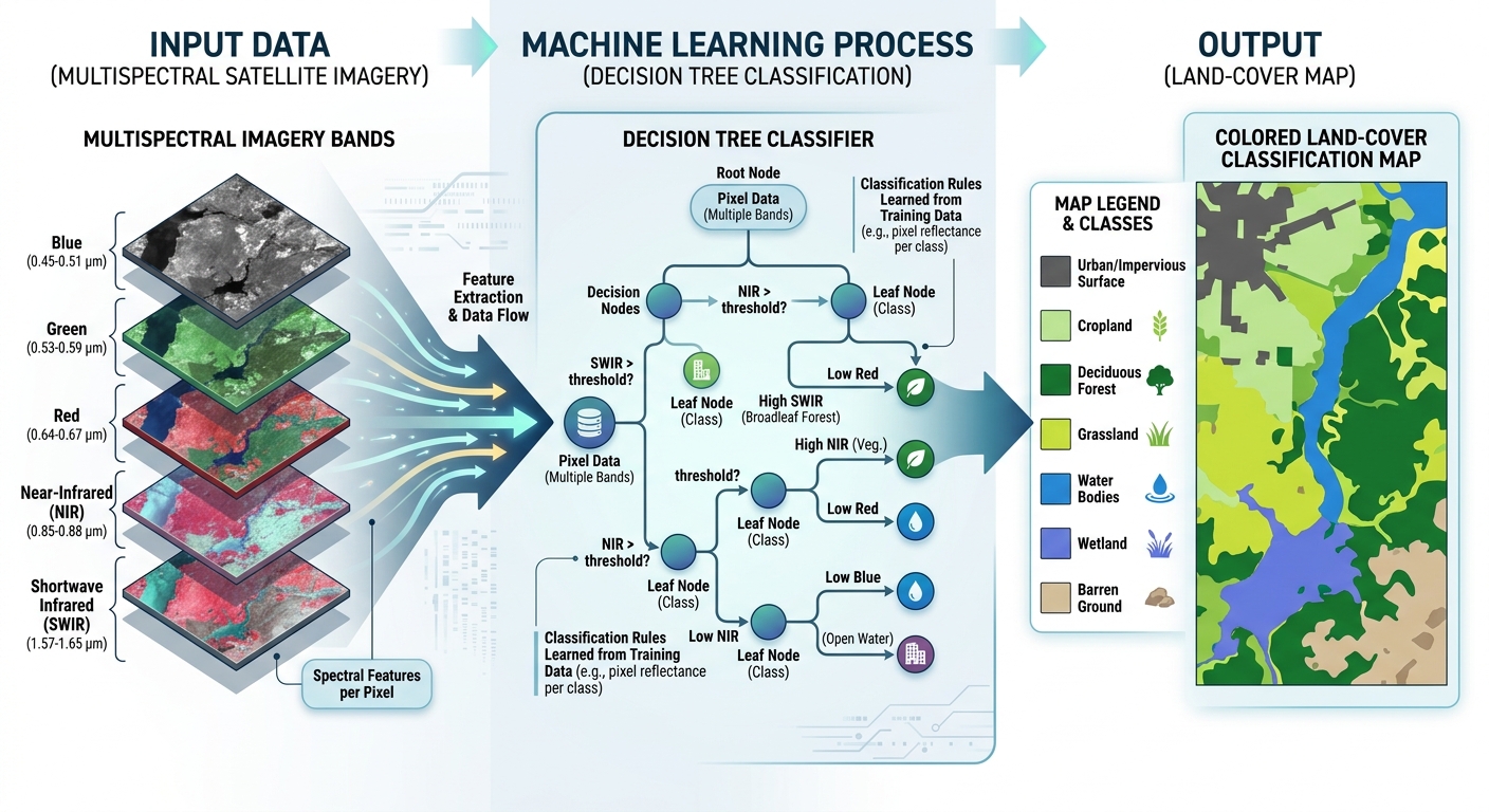
Random Forest Classification for Land Cover Mapping Using Python & GeoPandas
1. Introduction: Moving from Desktop GIS to Machine Learning
When exploring Random Forest Classification Python GIS land cover mapping is a fundamental application of remote sensing. It involves identifying surface categories such as forests, cropland, built-up areas, water bodies, and bare soil from satellite imagery.
Traditional GIS workflows often rely on visual interpretation, manual digitising, or rule-based spectral thresholds. These methods are useful, but they can become difficult to maintain when processing large satellite images, mapping multiple dates, or classifying several geographic regions.
Machine learning-based remote sensing classification offers an alternative. Instead of manually defining every classification rule, you provide labelled examples of known land-cover types and train an algorithm to recognise their spectral patterns.
One of the most widely used algorithms for this task is the Random Forest classifier.

What is Random Forest classification?
Random Forest is a supervised machine learning algorithm that combines predictions from many decision trees. Each tree learns classification rules from the training samples, and the forest combines their predictions to determine the final class.
For example, a classifier trained on multispectral satellite imagery may learn that:
- Water generally exhibits relatively low near-infrared reflectance.
- Healthy vegetation often has strong near-infrared reflectance.
- Built-up surfaces can exhibit distinctive visible, near-infrared, and shortwave-infrared responses.
- Bare soil and harvested fields may have spectral characteristics that differ from dense vegetation.
These are general patterns rather than universal rules. Soil moisture, vegetation condition, atmospheric effects, and sensor characteristics can cause different land-cover classes to overlap spectrally.
Random Forest can learn nonlinear relationships between spectral bands and, when provided, additional features such as vegetation indices, terrain variables, or seasonal observations.
Why use Python instead of relying only on GUI software?
Python allows you to build repeatable classification pipelines that can be automated, tested, and applied to large datasets.
This tutorial uses four primary libraries:
| Library | Role in the workflow |
|---|---|
| Rasterio | Reads satellite raster bands, handles masks, and writes classified GeoTIFFs |
| GeoPandas | Loads, inspects, and reprojects training polygons |
| NumPy | Manipulates raster arrays and prepares pixel-level training samples |
| scikit-learn | Trains the Random Forest model and evaluates classification accuracy |
The overall workflow is:
Multispectral satellite raster
              +
    Labelled training polygons
              |
              v
    Extract spectral signatures
              |
              v
   Split training and validation data
              |
              v
     Train Random Forest model
              |
              v
     Classify satellite pixels
              |
              v
      Export classified GeoTIFF
              |
              v
       Evaluate model accuracy
The tutorial uses an analysis-ready, multispectral raster with all input bands aligned to the same grid. Sentinel-2 or Landsat imagery can be used, provided the imagery is appropriately prepared and the training labels represent the land cover present at the time of acquisition.
2. Setting Up Your Python Environment
2.1 Install the required libraries
Proper preparation of your datasets is critical when implementing Random Forest Classification Python GIS land cover workflows to ensure clean feature extraction. Create a dedicated Python environment to keep your geospatial and machine learning dependencies organised.
Using Conda, you can create an environment with the required libraries:
conda create -n landcover python=3.12
conda activate landcover

conda install -c conda-forge \
    rasterio geopandas numpy pandas scikit-learn
Alternatively, in an existing compatible Python environment, install the packages using pip:
python -m pip install rasterio geopandas numpy pandas scikit-learnGeospatial libraries depend on native components such as GDAL, PROJ, and GEOS. Conda environments can simplify dependency management, especially for beginners.
Official documentation:
2.2 Prepare the satellite imagery
For this workflow, you need a multispectral raster containing the bands that will be used as classification features.
For example, Sentinel-2 imagery might contain:
- Blue.
- Green.
- Red.
- Near-infrared.
- Shortwave infrared bands.
The exact selection depends on the sensor, spatial resolution, and land-cover classes you want to distinguish.
Before running the classifier:
- Use suitable surface-reflectance imagery or another consistently processed satellite product.
- Mask clouds, cloud shadows, and invalid observations.
- Align all selected bands to the same coordinate reference system, pixel grid, and dimensions.
- Check band scaling and NoData values.
- Stack the bands into a multiband raster if they are stored in separate files.
Important: Sentinel-2 bands have different native spatial resolutions. Before stacking bands such as 10 m visible/NIR bands and 20 m SWIR bands, resample them to a common analysis grid. Resampling changes the grid representation, but it does not create new spatial information in the coarser bands.
For Sentinel-2, the Copernicus Data Space provides access to imagery. The USGS EarthExplorer provides access to Landsat imagery.
2.3 Prepare labelled training polygons
You also need a vector dataset containing polygons for known land-cover classes.
Create or collect polygons that represent categories such as:
| Class ID | Land-cover category | Example training location |
|---|---|---|
| 1 | Water | Lake or reservoir |
| 2 | Trees | Forest or woodland |
| 3 | Cropland | Agricultural fields |
| 4 | Built-up | Buildings and developed surfaces |
| 5 | Bare soil | Exposed soil or unvegetated ground |
These are example classes. Your categories should match the study area’s land-cover characteristics and the purpose of your project.
Save the training polygons in a format such as GeoPackage or Shapefile. Each polygon should have a label field, such as class_id, containing an integer class code.
Training polygons should represent the actual surface observed in the satellite image. Avoid polygons that cross multiple land-cover types, and resolve overlaps between polygons assigned to different classes.
For a reliable classification, collect multiple geographically distributed training polygons per class. A large number of pixels extracted from a single polygon does not substitute for diverse training locations.
3. Step-by-Step Code Walkthrough
The following implementation takes you from loading raster and vector data to training a classifier, predicting land cover, and exporting the final raster.
Step 1: Load multispectral raster bands and training polygons
First, import the necessary Python libraries and define the file paths.
from pathlib import Path

import numpy as np
import pandas as pd
import geopandas as gpd
import rasterio

from rasterio.mask import mask
from rasterio.windows import Window

from sklearn.ensemble import RandomForestClassifier
from sklearn.model_selection import train_test_split
from sklearn.metrics import (
    classification_report,
    confusion_matrix,
    accuracy_score,
)

# --------------------------------------------------
# File paths: replace these with your own files.
# --------------------------------------------------
RASTER_PATH = Path("data/sentinel2_stack.tif")
TRAINING_PATH = Path("data/training_polygons.gpkg")

OUTPUT_PATH = Path("output/landcover_random_forest.tif")

# Attribute containing the integer class code.
CLASS_FIELD = "class_id"

# Human-readable class labels.
CLASS_NAMES = {
    1: "Water",
    2: "Trees",
    3: "Cropland",
    4: "Built-up",
    5: "Bare soil",
}

# Number of pixels to retain per polygon during
# training sample extraction.
MAX_PIXELS_PER_POLYGON = 5000

# Create the output folder if it does not exist.
OUTPUT_PATH.parent.mkdir(parents=True, exist_ok=True)
The input raster is assumed to be a multiband GeoTIFF, where every band is already aligned to the same spatial grid.
Next, inspect the raster metadata and load the training polygons.
# --------------------------------------------------
# Inspect the satellite raster.
# --------------------------------------------------
with rasterio.open(RASTER_PATH) as src:
    if src.crs is None:
        raise ValueError("The satellite raster has no defined CRS.")

    raster_crs = src.crs

    print("Raster CRS:", raster_crs)
    print("Raster dimensions:", src.width, "x", src.height)
    print("Number of bands:", src.count)
    print("Pixel size:", src.res)
    print("Band descriptions:", src.descriptions)
    print("NoData value:", src.nodata)

# --------------------------------------------------
# Read training polygons using GeoPandas.
# --------------------------------------------------
training_gdf = gpd.read_file(TRAINING_PATH)

if training_gdf.crs is None:
    raise ValueError(
        "Training polygons have no CRS. "
        "Determine the correct CRS before continuing."
    )

if CLASS_FIELD not in training_gdf.columns:
    raise ValueError(
        f"Training polygons must contain '{CLASS_FIELD}'."
    )

# Remove missing or empty geometries and labels.
training_gdf = training_gdf.loc[
    training_gdf.geometry.notna()
    & ~training_gdf.geometry.is_empty
].dropna(subset=[CLASS_FIELD]).copy()

if training_gdf.empty:
    raise ValueError("No valid training polygons were found.")

# Convert class labels to integer codes.
training_gdf[CLASS_FIELD] = pd.to_numeric(
    training_gdf[CLASS_FIELD],
    errors="raise"
).astype(int)

# Reserve class 0 for NoData in the output raster.
if (training_gdf[CLASS_FIELD] <= 0).any():
    raise ValueError(
        "Class codes must be positive integers. "
        "Class 0 is reserved for NoData."
    )

# Reproject polygons to the raster CRS.
training_gdf = training_gdf.to_crs(raster_crs)

observed_classes = sorted(
    training_gdf[CLASS_FIELD].unique()
)

print("Training polygon count:", len(training_gdf))
print("Class codes:", observed_classes)
Why is CRS alignment important?
Rasterio uses the raster’s affine transform and coordinate system to determine which pixels overlap a geometry. GeoPandas’ to_crs() transforms vector coordinates into a new CRS.
If the training polygons and satellite raster use different CRSs, failing to reproject them can result in empty samples or incorrect pixel extraction.
Do not use set_crs() to repair a CRS mismatch unless the source CRS is genuinely missing or incorrectly labelled and you know the correct original reference system.
See the GeoPandas CRS documentation.
Step 2: Extract pixel spectral signatures from training polygons
This step converts your labelled polygons into the numerical feature matrix required by scikit-learn.
Suppose each pixel contains five spectral bands. A pixel’s spectral signature is represented by a feature vector:
[
X_i=[B_i,G_i,R_i,NIR_i,SWIR_i]
]
The corresponding label identifies the known land-cover category, such as water or cropland.
For supervised classification, the model receives pairs of feature vectors and known class labels:
[
\mathcal{D}={(X_i,y_i)}_{i=1}^{n}
]
Where:
- (X_i) represents the spectral features of pixel (i).
- (y_i) represents the known land-cover class.
- (n) is the number of training pixels.
The function below extracts valid pixel values from each training polygon. It excludes pixels masked by the raster’s NoData or internal mask information, as well as pixels containing non-finite values.
It also limits the number of pixels sampled per polygon, reducing the chance that one large training polygon dominates the training dataset.
def extract_polygon_samples(
    raster_path,
    polygons,
    class_field,
    max_pixels_per_polygon=5000,
    random_state=42,
):
    """
    Extract spectral samples from labelled polygons.

    Returns
    -------
    X : ndarray, shape (n_samples, n_bands)
        Pixel spectral features.
    y : ndarray, shape (n_samples,)
        Integer land-cover labels.
    """

    rng = np.random.default_rng(random_state)

    feature_arrays = []
    label_arrays = []

    with rasterio.open(raster_path) as src:
        for _, feature in polygons.iterrows():

            geometry = feature.geometry
            class_id = int(feature[class_field])

            # Extract the raster window intersecting this polygon.
            try:
                cropped, _ = mask(
                    src,
                    [geometry],
                    crop=True,
                    all_touched=False,
                    filled=False,
                )
            except ValueError:
                # This polygon may not overlap the raster.
                print(
                    f"Skipping non-overlapping polygon "
                    f"with class {class_id}."
                )
                continue

            # Masked array shape: (bands, rows, columns).
            raster_values = cropped.data

            # A pixel is invalid if any band is masked.
            invalid_mask = np.ma.getmaskarray(cropped).any(axis=0)

            # Rearrange to (rows, columns, bands).
            pixel_cube = np.moveaxis(raster_values, 0, -1)

            valid_mask = (
                ~invalid_mask
                & np.isfinite(pixel_cube).all(axis=-1)
            )

            # Keep only valid pixels inside this polygon.
            pixels = pixel_cube[valid_mask]

            if pixels.shape[0] == 0:
                print(
                    f"No valid pixels for polygon "
                    f"with class {class_id}."
                )
                continue

            # Limit samples from large polygons.
            if (
                max_pixels_per_polygon is not None
                and len(pixels) > max_pixels_per_polygon
            ):
                sample_idx = rng.choice(
                    len(pixels),
                    size=max_pixels_per_polygon,
                    replace=False,
                )
                pixels = pixels[sample_idx]

            feature_arrays.append(pixels)
            label_arrays.append(
                np.full(len(pixels), class_id, dtype=np.int32)
            )

    if not feature_arrays:
        raise ValueError(
            "No valid training pixels were extracted. "
            "Check raster coverage, masks, and CRS alignment."
        )

    X = np.vstack(feature_arrays)
    y = np.concatenate(label_arrays)

    return X, y


# Extract samples from all polygons initially.
X_all, y_all = extract_polygon_samples(
    RASTER_PATH,
    training_gdf,
    CLASS_FIELD,
    max_pixels_per_polygon=MAX_PIXELS_PER_POLYGON,
)

print("Feature matrix shape:", X_all.shape)
print("Label vector shape:", y_all.shape)
print("Samples per class:")
print(pd.Series(y_all).value_counts().sort_index())
Understanding the output
If the raster contains five bands and the function extracts 40,000 valid pixels, the feature matrix will have shape:
(40000, 5)The label vector will have shape:
(40000,)Each row in X_all contains one pixel’s spectral signature. The corresponding entry in y_all gives its training class.
The extraction uses all_touched=False, so Rasterio’s default geometry-mask behaviour generally includes pixels whose centres fall inside the polygon. Using all_touched=True includes every pixel touched by the polygon, which may be useful in some situations but can introduce more mixed pixels along boundaries.
For accurate training data, avoid polygon edges and mixed land-cover pixels where possible.
Rasterio documents its masking and feature extraction functions in the Rasterio mask reference.
Step 3: Split the data and train a Random Forest classifier
A common mistake is to use every training pixel both to fit the classifier and to evaluate its accuracy. This produces overly optimistic results because the model is tested on samples it has already encountered.
Remote sensing introduces another challenge: neighbouring pixels often have similar spectral values. If pixels from the same polygon are randomly distributed between training and test sets, the model may appear more accurate than it is when applied to new locations.
A stronger starting strategy is to split the training polygons into separate model-fitting and validation groups before extracting their pixels.
The code below reserves approximately 25% of the polygons for validation while attempting to preserve the class distribution.
Each class needs enough separate polygons for the split to work. For rigorous studies, allocate spatially distinct reference areas to validation or use spatially blocked validation so that neighbouring polygons do not appear in both subsets.
# --------------------------------------------------
# Check that each class has multiple polygons.
# --------------------------------------------------
polygon_counts = training_gdf[CLASS_FIELD].value_counts()

if (polygon_counts < 2).any():
    raise ValueError(
        "Each class needs at least two training polygons "
        "for this stratified polygon-level split."
    )

# Split polygons BEFORE extracting their pixel samples.
train_polygons, test_polygons = train_test_split(
    training_gdf,
    test_size=0.25,
    random_state=42,
    stratify=training_gdf[CLASS_FIELD],
)

# Extract model-fitting samples.
X_train, y_train = extract_polygon_samples(
    RASTER_PATH,
    train_polygons,
    CLASS_FIELD,
    max_pixels_per_polygon=MAX_PIXELS_PER_POLYGON,
    random_state=42,
)

# Extract validation samples from held-out polygons.
X_test, y_test = extract_polygon_samples(
    RASTER_PATH,
    test_polygons,
    CLASS_FIELD,
    max_pixels_per_polygon=MAX_PIXELS_PER_POLYGON,
    random_state=123,
)

print("Training samples:", X_train.shape[0])
print("Validation samples:", X_test.shape[0])
print("Training classes:", np.unique(y_train))
print("Validation classes:", np.unique(y_test))
The validation data must contain appropriate examples of every class you intend to evaluate. If the split leaves a class absent from the validation polygons, revise the geographic allocation or collect more reference polygons.
Train the model
Now configure the Random Forest classifier.
# --------------------------------------------------
# Configure and train the classifier.
# --------------------------------------------------
rf_model = RandomForestClassifier(
    n_estimators=300,
    max_features="sqrt",
    min_samples_leaf=1,
    class_weight="balanced_subsample",
    random_state=42,
    n_jobs=-1,
)

rf_model.fit(X_train, y_train)

print("Random Forest training completed.")
What do the parameters mean?
| Parameter | Explanation |
|---|---|
n_estimators=300 |
Trains 300 decision trees |
max_features="sqrt" |
Considers a square-root-based subset of features when searching for splits |
min_samples_leaf=1 |
Allows individual samples in terminal leaves; increase this value to encourage smoother decisions |
class_weight="balanced_subsample" |
Adjusts class weights separately for each tree’s bootstrap sample |
random_state=42 |
Makes the stochastic model fitting reproducible for the same data and software conditions |
n_jobs=-1 |
Uses available CPU cores for supported parallel operations |
Random Forest generally does not require feature standardisation, unlike algorithms that depend heavily on feature scale. Nevertheless, appropriate data cleaning, consistent band scaling, and careful handling of invalid pixels remain essential.
If your classes are severely imbalanced, consider class-specific sample limits, class weights, or carefully designed resampling. Do not allow the largest class to dominate simply because it occupies most of the image.
See the scikit-learn RandomForestClassifier documentation.
Step 4: Predict land cover across the entire raster grid
Once trained, the model can assign land-cover labels to previously unseen pixels.
Conceptually, the classifier applies the learned function to each valid pixel:
[
\boxed{\hat{y}i=f{\mathrm{RF}}(X_i)}
]
Where:
- (X_i) is the spectral feature vector for pixel (i).
- (f_{\mathrm{RF}}) is the trained Random Forest model.
- (\hat{y}_i) is the predicted class.
For a small raster, you could read all bands into memory and predict in one operation. However, larger satellite images can require substantial memory.
The following implementation predicts the image in blocks of 512 × 512 pixels. This reduces peak memory usage and allows you to classify larger GeoTIFFs without loading the entire image at once.
# --------------------------------------------------
# Prepare output data type.
# Class 0 is reserved for NoData.
# --------------------------------------------------
max_class_id = max(observed_classes)

if max_class_id <= 255:
    output_dtype = "uint8"
elif max_class_id <= 65535:
    output_dtype = "uint16"
else:
    raise ValueError(
        "Class IDs are too large for this example's "
        "integer GeoTIFF output configuration."
    )

if 0 in observed_classes:
    raise ValueError(
        "Class 0 is reserved for NoData in the output."
    )

# --------------------------------------------------
# Classify the raster window by window.
# --------------------------------------------------
with rasterio.open(RASTER_PATH) as src:

    output_profile = src.profile.copy()

    output_profile.update(
        driver="GTiff",
        count=1,
        dtype=output_dtype,
        nodata=0,
        compress="lzw",
    )

    with rasterio.open(
        OUTPUT_PATH,
        "w",
        **output_profile,
    ) as dst:

        block_size = 512

        for row_off in range(0, src.height, block_size):
            for col_off in range(0, src.width, block_size):

                window = Window(
                    col_off,
                    row_off,
                    min(block_size, src.width - col_off),
                    min(block_size, src.height - row_off),
                )

                # Read the current raster block with masks.
                block = src.read(
                    window=window,
                    masked=True,
                )

                # Shape: (bands, rows, columns).
                block_values = block.data

                # A pixel is valid only when every input band
                # is unmasked and all values are finite.
                valid_mask = (
                    ~np.ma.getmaskarray(block).any(axis=0)
                    & np.isfinite(block_values).all(axis=0)
                )

                # Move the band axis to the final position.
                # Shape becomes (rows, columns, bands).
                pixel_matrix = np.moveaxis(
                    block_values,
                    0,
                    -1,
                )

                # Reserve class 0 for invalid pixels.
                prediction = np.zeros(
                    valid_mask.shape,
                    dtype=output_dtype,
                )

                if valid_mask.any():

                    # Predict only valid pixels.
                    valid_pixels = pixel_matrix[valid_mask]

                    predicted_classes = rf_model.predict(
                        valid_pixels
                    )

                    prediction[valid_mask] = predicted_classes

                # Write the classified block.
                dst.write(
                    prediction,
                    1,
                    window=window,
                )

print(f"Classification saved to: {OUTPUT_PATH}")
Why classify in blocks?
A raster containing 10,000 × 10,000 pixels has 100 million cells. A five-band image requires at least 500 million band values before additional arrays and intermediate calculations are considered.
Block processing allows the classifier to load a manageable section, predict its valid pixels, and write the result before moving to the next section.
The code retains the original raster’s CRS, affine transform, and dimensions through its profile, while changing the output to a single-band integer GeoTIFF.
Rasterio’s writing datasets documentation explains how dataset profiles are used to create correctly georeferenced outputs.
Quality check: Load the output raster into QGIS and compare it with the input imagery. Confirm that class boundaries align spatially, that invalid areas are represented as NoData, and that the output codes correspond to your land-cover legend.
Step 5: Evaluate classification accuracy
A visually convincing land-cover map is not necessarily accurate. Some land-cover classes have similar spectral signatures, while clouds, shadows, seasonal changes, and mixed pixels can create confusion.
Evaluate the classifier using the withheld validation polygons—not the training pixels.
5.1 Generate a classification report
Predict the validation samples and calculate the classification report.
# --------------------------------------------------
# Predict the held-out validation samples.
# --------------------------------------------------
y_pred = rf_model.predict(X_test)

class_ids = sorted(
    set(observed_classes)
    | set(np.unique(y_test))
    | set(np.unique(y_pred))
)

target_names = [
    CLASS_NAMES.get(class_id, f"Class {class_id}")
    for class_id in class_ids
]

# --------------------------------------------------
# Print overall accuracy.
# --------------------------------------------------
overall_accuracy = accuracy_score(y_test, y_pred)

print(f"Overall accuracy: {overall_accuracy:.3f}")

# --------------------------------------------------
# Print per-class performance.
# --------------------------------------------------
print(
    classification_report(
        y_test,
        y_pred,
        labels=class_ids,
        target_names=target_names,
        zero_division=0,
    )
)
The classification report includes several important metrics.
| Metric | Meaning |
|---|---|
| Precision | Of the pixels predicted as a class, the proportion that actually belongs to that class |
| Recall | Of the reference pixels belonging to a class, the proportion correctly identified |
| F1-score | Harmonic mean of precision and recall |
| Support | Number of validation samples belonging to each reference class |
| Overall accuracy | Proportion of all validation samples classified correctly |
For example, high precision for the water class means that few validation pixels predicted as water belong to other reference classes. High recall for water means that most reference water pixels are detected.
Overall accuracy can conceal poor performance in minority classes. Always examine the per-class metrics, especially if certain land-cover categories occupy only a small percentage of the study area.
5.2 Generate a confusion matrix
A confusion matrix makes it easier to identify which classes are being mistaken for one another.
# --------------------------------------------------
# Build a confusion matrix.
# Rows = actual classes.
# Columns = predicted classes.
# --------------------------------------------------
cm = confusion_matrix(
    y_test,
    y_pred,
    labels=class_ids,
)

confusion_df = pd.DataFrame(
    cm,
    index=[f"Actual: {name}" for name in target_names],
    columns=[f"Predicted: {name}" for name in target_names],
)

print(confusion_df)
Suppose the model frequently confuses cropland with bare soil. This may indicate that the training imagery was acquired when fields were harvested or that the spectral information does not clearly distinguish the two classes.
Possible improvements include collecting better training samples, adding seasonal imagery, incorporating near-infrared or shortwave-infrared features, and reviewing the class definitions.
See the official scikit-learn classification metrics documentation.
5.3 Avoid spatial validation leakage
The validation strategy strongly affects how you should interpret the reported accuracy.
A random split of individual pixels is usually inappropriate for land-cover mapping because nearby pixels often have similar spectral signatures. Even a random split of polygons may be optimistic if training and validation polygons are immediately adjacent or represent the same homogeneous field.
For more rigorous evaluation:
- Separate geographically distinct reference sites or spatial blocks before fitting the model.
- Use only the training regions to fit the classifier.
- Evaluate it on independent regions that were not used for model selection.
- Where possible, use independent field observations or reference data from another source.
- Report the sampling method, class distribution, assessment period, and limitations.
A random polygon split is a useful starting point for this tutorial, but spatially independent validation is preferable when the objective is to estimate performance in new areas.
The scikit-learn guidance on model validation and common pitfalls explain why testing on data that are too similar to the training set can overestimate generalisation.
Step 6: Inspect feature importance
Random Forest can provide a ranking of how useful each input feature was for reducing impurity across the fitted trees.
This can offer insight into which bands contributed most to the model’s decisions.
# --------------------------------------------------
# Inspect impurity-based feature importance.
# --------------------------------------------------
with rasterio.open(RASTER_PATH) as src:
    band_names = [
        description or f"Band_{i}"
        for i, description in enumerate(src.descriptions, start=1)
    ]

importance_df = pd.DataFrame({
    "band": band_names,
    "importance": rf_model.feature_importances_,
})

importance_df = importance_df.sort_values(
    "importance",
    ascending=False,
)

print(importance_df)
The feature names in the raster metadata should describe the same band order used during training.
Feature importance is not a causal explanation of land-cover processes, and correlated spectral bands can share or redistribute importance. Use it as a diagnostic rather than treating the highest-ranked band as universally the most important for land-cover classification.
For a more robust interpretation, consider permutation importance on an independent validation set.
4. Improving the Classification Workflow
The basic Random Forest pipeline is a starting point. Several improvements may be appropriate for research-grade mapping. Advanced practitioners looking to scale up their Random Forest Classification Python GIS land cover pipeline can also incorporate multi-temporal satellite observations.
4.1 Add vegetation indices
Vegetation indices can complement raw reflectance bands.
For example, NDVI is calculated as:
[
\mathrm{NDVI}=\frac{NIR-Red}{NIR+Red}
]
You can add NDVI as an additional feature if the index is computed consistently for both the training samples and the raster pixels being classified.
Use an explicit feature stack so that the model receives identical features in identical order during training and prediction.
4.2 Incorporate seasonal or temporal information
Some classes are difficult to distinguish in a single satellite image. A field may resemble bare soil after harvest but exhibit a strong vegetation response several weeks later.
Combining observations from multiple dates can improve separability between crops, natural vegetation, and other land-cover classes, provided the images are co-registered and comparably processed.
4.3 Tune Random Forest parameters
You can investigate the effect of:
n_estimators: Number of trees.max_features: Number or fraction of features considered at each split.max_depth: Maximum tree depth.min_samples_leaf: Minimum number of samples per terminal leaf.class_weight: How class imbalance is handled.
Tune these parameters using training data and an appropriate validation strategy. Do not repeatedly modify parameters based on the final independent test set, because this leaks evaluation information into model selection.
4.4 Consider uncertainty and classification probabilities
Random Forest can return class probabilities through predict_proba(). These values can be useful for identifying ambiguous pixels, but they should not automatically be interpreted as calibrated probabilities that the land-cover label is correct.
A useful quality-assessment product can combine:
- The final classified map.
- A per-pixel confidence or maximum probability layer.
- The validation report and confusion matrix.
- A map of areas with low confidence or poor training coverage.
This can help direct additional fieldwork and review toward uncertain areas.
5. Common Technical Errors to Avoid
Misaligned raster bands: If the bands do not share the same grid, the feature vectors may combine values from different ground locations. Align the bands before training and prediction.
Incorrect training labels: A polygon labelled as forest may contain roads or clearings. Inspect training areas carefully and avoid mixed-class polygons.
NoData and cloud contamination: Invalid or cloudy pixels can enter the classifier if they are not masked consistently. Ensure that invalid cells are excluded from training and assigned NoData in the output.
Insufficient training diversity: A model trained on a few isolated examples may perform well locally but fail in unfamiliar areas. Sample each class across representative locations and conditions.
Class imbalance: Overall accuracy may appear high when a dominant class is classified correctly but rare classes perform poorly. Use per-class metrics and assess the sampling design.
Random pixel validation: Nearby pixels can be highly correlated, inflating apparent performance. Prefer independent polygons or spatial blocks for assessment.
Incorrect output data type: The class-code raster must use an integer type that can represent every class value. In this example, class 0 is reserved for NoData, so valid class IDs must be positive.
6. Conclusion
Random Forest classification provides a flexible, repeatable method for producing land-cover maps from multispectral satellite imagery. With Rasterio for raster management, GeoPandas for vector training data, NumPy for pixel processing, and scikit-learn for model fitting, a GIS analyst can build an end-to-end classification pipeline in Python.
The workflow begins by preparing and aligning satellite imagery, extracting spectral signatures from labelled polygons, separating training and validation areas, training the classifier, and predicting land cover in memory-efficient raster blocks. The final GeoTIFF can then be loaded into QGIS or ArcGIS Pro for mapping, area calculations, change analysis, and reporting.
For reliable research, the most important lesson is that classification quality depends on both the model and the quality of the reference data and validation design. A sophisticated algorithm cannot compensate for poor labels, inconsistent imagery, or an evaluation that uses samples too similar to those used in training. By following this guide on Random Forest Classification Python GIS land cover, you can build a repeatable and robust machine learning workflow using Python. Mastering these technical fundamentals of Random Forest Classification Python GIS land cover empowers you to automate large-scale environmental monitoring projects using Python.
Further Resources
- Rasterio Documentation — Reading, masking, processing, and writing raster datasets.
- GeoPandas Documentation — Loading and managing labelled training polygons.
- scikit-learn RandomForestClassifier — Model parameters and prediction methods.
- scikit-learn Classification Metrics — Classification reports, confusion matrices, and evaluation metrics.
- Copernicus Data Space — Access Sentinel-2 imagery.
- USGS EarthExplorer — Access Landsat imagery and other remote sensing datasets.