Anselin Local Moran’s I (LISA) in GIS: How to Identify Spatial Outliers & Clusters

 

1. Introduction: What Is Local Moran’s I (LISA)?

When using Anselin Local Morans I LISA GIS, Imagine you are mapping household income across 100 urban neighborhoods. Most neighborhood’s have similar income levels to their neighbors, but a few stand out. One wealthy neighborhood is surrounded by lower-income areas, while another group of wealthy neighborhoods forms a larger high-income cluster.

A conventional choropleth map can show these differences, but it does not tell you whether each location exhibits a statistically significant local spatial pattern.

Anselin Local Moran’s I is a spatial statistics method designed to identify local clusters and spatial outliers. It belongs to a broader family of methods called Local Indicators of Spatial Association (LISA), introduced by Luc Anselin to examine local spatial associations and how individual locations contribute to broader spatial patterns.

LISA statistics help answer a question that a global spatial statistic cannot answer by itself:

Where in the study area are similar or contrasting values spatially associated?

Local Moran’s I can identify neighbourhoods where high values occur beside high values, low values occur beside low values, or an unusually high or low value occurs among neighbours with contrasting values.

Common applications include:

• Crime analysis: Identifying areas with clustered crime rates and neighbourhoods that differ from their surroundings.
• Housing research: Detecting clusters of high or low property prices and unusual neighbourhoods.
• Public health: Examining spatial clusters of disease rates.
• Environmental analysis: Finding clusters of high pollution measurements or unusually low vegetation values.
• Regional development: Investigating geographically concentrated income, unemployment, or deprivation.

The method is available through the ArcGIS Pro Cluster and Outlier Analysis tool, open-source QGIS plugins, and Python libraries such as PySAL’s esda package.

2. Global Moran’s I vs. Local Moran’s I

Before performing local analysis, it helps to understand the difference between global and local spatial autocorrelation.

Global Moran’s I summarizes the overall spatial association of a variable across the entire study area. Its result indicates whether similar or contrasting values tend to be spatially associated overall.

Local Moran’s I calculates a local statistic for each feature, helping to identify where specific clusters and outliers occur.

Feature	Global Moran’s I	Anselin Local Moran’s I
Main question	Is there overall spatial autocorrelation?	Where are the local clusters and spatial outliers?
Output	One principal global statistic	Local statistics for individual features
Identifies local outliers?	No	Yes
Identifies High–High and Low–Low patterns?	Not individually	Yes
Statistical significance	Overall test	Local test for each feature
Typical application	Testing for a general spatial pattern	Locating clusters and unusual observations

For example, a positive Global Moran’s I result for household income suggests that similar income values tend to be spatially associated. However, it cannot independently identify the precise neighbourhoods forming high-income clusters.

Local Moran’s I provides that additional spatial detail. A study can use both methods: begin with an overall assessment and then investigate local patterns relevant to the research question. PySAL’s Local Spatial Autocorrelation guide explains this distinction. When comparing global and local patterns, Anselin Local Morans I LISA GIS techniques reveal spatial nuances that global metrics miss.

3. Understanding the Four Local Moran’s I Cluster Types

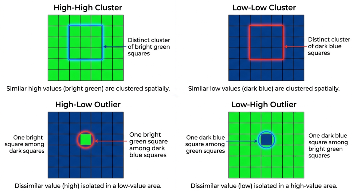
The main advantage of Local Moran’s I is that it distinguishes four local spatial patterns. These are determined by the relationship between an observation’s value and the values of its neighbours.

A useful way to understand the patterns is to compare each feature’s value with the study-area average, then examine whether its neighbours tend to have relatively high or low values. Understanding the four quadrant types is essential when applying Anselin Local Morans I LISA GIS for granular spatial data exploration.

3.1 High–High (HH): Clusters of high values

A High–High cluster occurs when a feature has a high value relative to the overall distribution and its neighbours also tend to have high values.

For example, a group of adjacent neighbourhoods may all have relatively high average household incomes. Local Moran’s I may identify these neighbourhoods as a statistically significant High–High cluster.

Other examples include:

• Areas with high housing prices surrounded by other high-price areas.
• Districts with high crime rates near other high-crime districts.
• Regions with high pollution measurements surrounded by similarly polluted regions.

HH clusters are often described as local high-value clusters or hotspots. However, a High–High result from Local Moran’s I is not identical to a hotspot detected using Getis-Ord Gi*. The statistical methods test related but different forms of spatial concentration.

Interpretation: The feature has a high value, and its neighbours tend to have high values as well.

3.2 Low–Low (LL): Clusters of low values

A Low–Low cluster occurs when a feature has a relatively low value and its neighbouring features also tend to have low values.

For example, several neighbouring neighbourhoods may have consistently low housing prices relative to the study-area average.

Other applications include:

• Areas with low recorded disease incidence.
• Districts with low average income.
• Regions with low measured pollution levels.
• Locations with low vegetation index values.

LL clusters are sometimes called cold spots when low values represent the phenomenon of interest. The interpretation depends on the variable. A cluster of low disease incidence may be favourable, while a cluster of low rainfall may be a drought concern.

Interpretation: The feature has a low value, and its neighbours tend to have low values as well.

3.3 High–Low (HL): High-value spatial outliers

A High–Low outlier occurs when a feature has a relatively high value but its neighbouring features tend to have low values.

Imagine a high-income neighbourhood surrounded mainly by lower-income neighbourhoods. Local Moran’s I may classify it as an HL outlier if the pattern is statistically significant.

Other examples include:

• A district with an unusually high crime rate among lower-crime neighbours.
• A highly polluted site surrounded by locations with relatively low pollution.
• An expensive housing area surrounded by comparatively inexpensive neighbourhoods.

A High–Low feature deserves attention because its values contrast with the surrounding spatial context. The outlier could reflect a real local difference, a special land use, or an unusual measurement.

It could also result from incorrect data, an unusual polygon boundary, or an inappropriate spatial weights definition.

Interpretation: The feature has a high value relative to the dataset, but its neighbours tend to have low values.

3.4 Low–High (LH): Low-value spatial outliers

A Low–High outlier occurs when a feature has a relatively low value and its neighbours tend to have high values.

For example, an affordable neighbourhood may be surrounded by much more expensive areas.

Other examples include:

• A low-crime district surrounded by high-crime districts.
• A low-pollution location within a region of higher pollution.
• An area of low vegetation cover surrounded by locations with relatively high vegetation values.

These locations may warrant further investigation, especially when the surrounding pattern is important to planning or environmental management.

Interpretation: The feature has a low value relative to the dataset, but its neighbours tend to have high values.

Quick reference: The four patterns

Cluster type	Feature value	Neighbour values	Meaning
High–High (HH)	High	High	Cluster of similar high values
Low–Low (LL)	Low	Low	Cluster of similar low values
High–Low (HL)	High	Low	High-value spatial outlier
Low–High (LH)	Low	High	Low-value spatial outlier

Important: These labels are meaningful as statistical findings only when the relevant local test is significant. A high-valued feature surrounded by lower values is not automatically a statistically significant HL outlier.

4. Step 1: Select and Prepare the Attribute Data

Before opening a spatial statistics tool, ensure your dataset is suitable for local spatial analysis.

For this example, suppose you want to identify clusters and outliers in household income across administrative neighbourhoods.

4.1 Choose the right analysis variable

Suitable variables include:

• Mean or median household income.
• Housing price per square metre.
• Crime rate per 1,000 or 100,000 residents.
• Disease incidence rate.
• Annual average pollution concentration.
• Vegetation index values.

The variable should be numerical and should contain meaningful variation across features.

For crime analysis, avoid assuming that raw crime counts are directly comparable across neighbourhoods of very different population sizes. A rate or another justified population-adjusted measure may be more appropriate, depending on your research question.

Likewise, if you are comparing disease incidence, consider whether differences in population size, age structure, or reporting practices could influence the observed pattern.

4.2 Check the spatial dataset

Before analysis:

• Confirm that each feature represents one meaningful observation, such as one administrative neighbourhood.

• Inspect the attribute table for missing or invalid values.

• Check for duplicate features and duplicate records.

• Verify that the input field has numerical variation.

• Confirm that the geometry is valid and the study area is defined consistently.

• Check the coordinate reference system.

• Verify that each feature can be connected to neighbouring features through the chosen spatial relationships.

If your dataset contains hundreds of crime incident points, consider whether the research question is better addressed by aggregating incidents into suitable areas or using an event-based hotspot method. Local Moran’s I is most directly interpretable when each analysed feature has an attribute value with meaningful local neighbourhood relationships.

4.3 Understand why spatial weights matter

Local Moran’s I depends on a spatial weights matrix. This matrix defines which features are neighbours and how strongly they influence the local calculation.

The same income dataset can produce different LISA patterns under different neighbourhood definitions. That is not necessarily an error; the analysis is answering a slightly different spatial question.

Before running the tool, decide how neighbourhood relationships should be represented.

5. Step 2: Define Spatial Relationships and Distance Bands

A spatial weights matrix formalizes the concept of neighbourhood. It can use shared polygon boundaries, distances between points or feature centroids, or a specified number of nearest neighbours. Selecting the correct spatial weights matrix is a critical technical step in any robust Anselin Local Morans I LISA GIS workflow.

5.1 Contiguity-based weights

Contiguity is commonly used for polygon datasets such as administrative boundaries.

• Rook contiguity: Two polygons are neighbours when they share an edge.
• Queen contiguity: Two polygons are neighbours when they share an edge or a corner.

These definitions are useful when the research question concerns adjacent administrative areas.

For example, if your study uses district polygons, you may consider Queen contiguity when areas touching at a corner should count as neighbours, or Rook contiguity when a shared boundary is required.

5.2 Fixed Distance Band

A fixed distance band defines neighbours using a specified cutoff distance. Features inside the chosen threshold receive a spatial weight, while those outside are treated as non-neighbours under that model.

This is useful when distance represents a meaningful geographic relationship, such as the local context around monitoring stations or neighbourhood centroids.

Choose the threshold carefully. If it is too small, some features may have no neighbours. If it is too large, the analysis may combine locations whose interactions are not meaningful for the research question.

5.3 K-nearest neighbours

The K-nearest neighbours method defines each feature’s neighbours by selecting the closest (k) features.

This can be helpful when features are unevenly distributed and a fixed distance would leave some features isolated.

However, it imposes a consistent neighbour count rather than a consistent geographic distance. In sparse areas, the selected neighbours may be much farther away than those in dense areas.

5.4 Inverse distance weights

Inverse distance weighting assigns more influence to nearby features and less influence to more distant features.

It is useful when geographic influence is expected to decline with distance rather than stop at a sharp cutoff.

The weight structure should reflect a plausible spatial process, not simply a parameter setting that produces a visually attractive map.

How should a student choose?

Dataset or question	Reasonable starting point
Adjacent administrative polygons	Rook or Queen contiguity
Point observations with a meaningful interaction distance	Fixed distance band
Unevenly distributed points where every feature needs neighbours	K-nearest neighbours
Relationships expected to weaken gradually with distance	Inverse distance weights

For distance-based weights, use a suitable projected coordinate reference system when possible so the distances and thresholds are expressed in meaningful units. The ArcGIS Pro documentation explains these alternatives in the Cluster and Outlier Analysis tool reference.

Best practice: Record the weights method, threshold or number of neighbours, and standardization choice in your methodology. Where the study design permits, test whether the main findings persist under another defensible neighbourhood definition.

6. Step 3: Run Local Moran’s I in ArcGIS Pro

ArcGIS Pro includes a tool called Cluster and Outlier Analysis (Anselin Local Moran’s I). It calculates the local Moran’s I index, a Z-score, a p-value, and a cluster/outlier classification for each feature. Official tool documentation.

Procedure

1. Prepare the feature layer

• Open your ArcGIS Pro project.
• Add the polygon or point dataset containing the variable you want to analyse.
• Inspect the attribute table and verify the analysis field.
• Confirm the coordinate system and check for missing values.

2. Open the geoprocessing tool

• Click Analysis → Tools.
• Search for Cluster and Outlier Analysis (Anselin Local Moran’s I).
• Open the tool.

3. Configure the main parameters

• Input Feature Class: Select the dataset containing the spatial features.
• Input Field: Select the numeric attribute, such as MEDIAN_INCOME.
• Output Feature Class: Specify where the result should be saved.
• Conceptualization of Spatial Relationships: Choose a suitable weights method, such as polygon contiguity, fixed distance band, inverse distance, or K-nearest neighbours.
• Distance Band or Threshold Distance: Enter a justifiable cutoff where required.
• Standardization: Choose row standardization when appropriate for the weights structure and sampling or aggregation design.
• Number of Permutations: Use enough permutations for the required statistical precision. The tool’s default is 499; larger counts can provide finer pseudo-p-value resolution at additional computational cost.
• Apply False Discovery Rate (FDR) Correction: Consider enabling this when testing many features, to account for multiple local significance tests.

The exact fields available depend on the selected spatial relationship method. If you use polygon contiguity, for example, a distance-band parameter does not define the relationships.

4. Run the tool

• Review all parameters.
• Click Run.
• Wait for processing to finish.
• Inspect the output feature class in the Contents pane.

5. Review the result fields

ArcGIS Pro outputs a local Moran’s I index, a Z-score, a p-value, and a cluster/outlier type field commonly called COType. The output may also include a source identifier used to relate results to the original features. Only statistically significant features receive a cluster/outlier classification in the standard output workflow. In ArcGIS Pro, executing Anselin Local Morans I LISA GIS allows analysts to generate localized cluster and outlier maps efficiently.

What should the output look like?

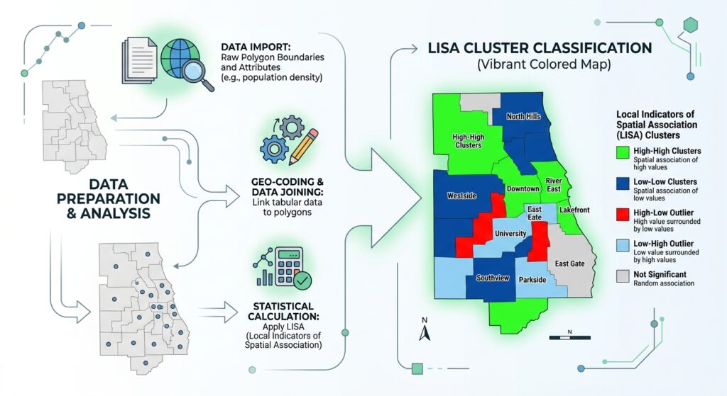
The software typically applies default symbology to the cluster/outlier classification. You can refine the colours and legend to distinguish High–High, Low–Low, High–Low, Low–High, and non-significant features.

Do not interpret an empty COType field as a fifth cluster category. In this workflow, an empty classification can indicate that a feature did not meet the statistical significance threshold. Features with no neighbours may have a separate code such as NN. Check the output documentation and attribute values for the version you are using.

7. Step 4: Run Local Moran’s I in QGIS

QGIS provides a flexible open-source route, although Local Moran’s I is not part of the same standard built-in toolset as ArcGIS Pro’s named Cluster and Outlier Analysis tool. For open-source users, implementing Anselin Local Morans I LISA GIS via Python libraries like PySAL provides complete automation flexibility.

There are two practical approaches: use a compatible QGIS Processing plugin, or use Python with GeoPandas and PySAL.

Option A: Use the QGIS Hotspot Analysis plugin

The QGIS plugin repository lists Hotspot Analysis v3, which provides Processing algorithms for univariate Local Moran’s I, bivariate Local Moran’s I, and Getis-Ord Gi*. Check the listing for the version supported by your installation. Official QGIS plugin listing.

Procedure

1. Prepare the dataset

• Open your QGIS project.
• Add the polygon or point layer containing the variable to be analysed.
• Confirm that the numeric field is populated and that the coordinate reference system is appropriate.
• Check geometries, missing data, duplicate features, and the intended spatial weights.

2. Install the plugin

• Click Plugins → Manage and Install Plugins.
• Search for Hotspot Analysis v3.
• Review the plugin information and compatibility.
• Install the plugin if it is appropriate for your QGIS version and project requirements.

3. Open the Local Moran’s I algorithm

• Open the Processing Toolbox.
• Search for the univariate Local Moran’s I algorithm provided by the plugin.
• Select the prepared input layer and numerical variable.
• Configure the supported spatial weights or neighbourhood parameters.
• Set permutation and significance options where available.
• Select an output location and run the tool.

The names and parameters may differ with plugin versions. Read the algorithm help and verify its implementation and output fields before comparing its results with another package.

4. Inspect the output

• Open the output attribute table.
• Identify the local statistic, significance information, and cluster/outlier classification.
• Style High–High and Low–Low clusters separately from High–Low and Low–High outliers.
• Check whether non-significant features are distinguished clearly.

Option B: Use GeoPandas and PySAL

For students interested in open-source spatial programming, PySAL’s esda package provides Local Moran’s I statistics, while libpysal creates spatial weights and GeoPandas manages the spatial table.

The official PySAL Local Moran’s I tutorial demonstrates the approach.

First, install the required libraries in a compatible Python environment:

pip install geopandas libpysal esda

The following example uses Queen contiguity for polygon features and assumes that your input file contains a numeric field called MEDIAN_INCOME.

import geopandas as gpd
from libpysal.weights import Queen
from esda import Moran_Local

# Load the polygon dataset
gdf = gpd.read_file("data/neighbourhoods.gpkg")

# Retain only rows with usable income values
gdf = gdf.dropna(subset=["MEDIAN_INCOME"]).copy()

# Create Queen-contiguity spatial weights
w = Queen.from_dataframe(gdf)

# Check whether any polygons have no neighbours
if w.islands:
    print("Features without neighbours:", w.islands)

# Row-standardize the spatial weights
w.transform = "R"

# Retrieve the numeric attribute
y = gdf["MEDIAN_INCOME"].to_numpy()

# Calculate Local Moran's I using 999 permutations
lisa = Moran_Local(
    y,
    w,
    permutations=999,
    geoda_quads=True,
    seed=42
)

# Store the local statistics and pseudo p-values
gdf["local_I"] = lisa.Is
gdf["p_value"] = lisa.p_sim
gdf["quadrant"] = lisa.q

# Translate the GeoDa-style quadrant codes
cluster_labels = {
    1: "High-High",
    2: "Low-Low",
    3: "Low-High",
    4: "High-Low"
}

gdf["cluster_type"] = gdf["quadrant"].map(cluster_labels)

# Keep a classification only for significant observations.
# This unadjusted threshold is an example, not a multiple-testing correction.
gdf.loc[gdf["p_value"] >= 0.05, "cluster_type"] = "Not significant"

# Export the results
gdf.to_file(
    "outputs/local_morans_results.gpkg",
    layer="local_morans",
    driver="GPKG"
)

print(gdf[["MEDIAN_INCOME", "local_I", "p_value",
           "cluster_type"]].head())

Before using this script in a thesis, note three things:

• The code assumes that the retained records, the weights matrix, and the attribute array remain in the same order. Avoid reordering one of them independently.
• Queen contiguity is suitable for adjoining polygons; point data or non-contiguous features may need a different weights structure. Investigate and handle features without neighbours rather than assuming they are harmless.
• The example uses an unadjusted (p < 0.05) threshold. For analyses involving many features, consider multiple-testing correction and document the method used.

Also check the PySAL documentation for the interpretation of quadrant codes. The code above explicitly uses geoda_quads=True so that the mapping of quadrants to HH, LL, LH, and HL follows the GeoDa convention. PySAL Moran_Local reference.

This approach provides an auditable workflow and lets you repeat the same analysis on different datasets. However, it remains your responsibility to justify the weights, inspect the output, and verify that the assumptions are appropriate for your research.

8. Step 5: Interpret Local Moran’s I, Z-Scores, and P-Values

Local Moran’s I output commonly includes three statistical quantities and a cluster/outlier classification. Each has a different purpose.

8.1 Local Moran’s I index

The local Moran’s I index measures the direction and relative strength of local spatial association under the specified weights structure.

• A positive local I typically indicates similarity between the target feature and its weighted neighbours, consistent with HH or LL patterns.
• A negative local I typically indicates dissimilarity between the target feature and its neighbours, consistent with HL or LH patterns.

Do not interpret the index by itself. Its magnitude depends on the data and weights, and its statistical significance must be considered with the associated inference results.

8.2 Z-score

The Z-score expresses the observed local statistic relative to its expected value and variability under the chosen statistical model.

A large positive Z-score may indicate a significant local cluster, while a sufficiently negative Z-score may indicate a significant spatial outlier. The classification into HH, LL, HL, or LH then depends on the observation’s value and its neighbourhood context.

The Z-score is not the same as the raw income value, crime rate, or pollution measurement. It is a standardized statistical quantity used to assess the evidence for a local pattern.

8.3 P-value and permutation-based inference

A P-value measures the strength of evidence against the null hypothesis for an individual local test, subject to the assumptions of the statistical procedure.

In permutation-based Local Moran’s I, the software constructs a reference distribution by randomly rearranging values according to its permutation procedure, recalculating the local statistic, and comparing the observed result to that distribution.

ArcGIS Pro uses permutation-based pseudo p-values by default, with 499 permutations unless changed. Increasing the number of permutations allows finer p-value resolution but takes more time. ArcGIS Pro’s methodology documentation explains the calculation and interpretation.

An ordinary significance threshold of (p < 0.05) is common, but testing hundreds of features creates a multiple-comparisons problem: some areas may appear significant simply by chance.

For local analyses, consider False Discovery Rate (FDR) correction or another justified multiple-testing approach. ArcGIS Pro offers FDR correction in its Cluster and Outlier Analysis tool; in Python, choose and document a suitable correction method if required.

Example interpretation table

Local pattern	Illustrative evidence	Interpretation
HH	High-valued feature, high-valued neighbours, significant local test	Statistically significant cluster of high values
LL	Low-valued feature, low-valued neighbours, significant local test	Statistically significant cluster of low values
HL	High-valued feature, low-valued neighbours, significant local test	Statistically significant high-value outlier
LH	Low-valued feature, high-valued neighbours, significant local test	Statistically significant low-value outlier
Not significant	Local test does not meet the selected threshold	Insufficient evidence to classify the feature under the chosen model

A non-significant result does not prove that a feature has no spatial relationship with its neighbours. It means the analysis has not found sufficient evidence to classify its local pattern as statistically significant under the selected model and threshold.

9. Practical Application: Finding a High-Income Neighbourhood

Consider a hypothetical study of 80 neighbourhoods. Each polygon has a median household income value, and the analysis uses Queen contiguity to define neighbouring areas.

After running Local Moran’s I, suppose one neighbourhood has the following illustrative results:

Output	Example result
Median household income	85,000
Local Moran’s I	−0.42
Z-score	−2.70
P-value	0.008
Cluster type	High–Low

These values are hypothetical, not results from an actual dataset.

The interpretation is that the neighbourhood has a relatively high income compared with the study-area distribution, while its neighbouring areas tend to have relatively low income. The negative local statistic and statistically significant result support classification as a High–Low spatial outlier under the chosen model.

What might explain the pattern? Possible explanations could include a gated development, a business district with residential properties, a recent housing development, or differences in local land use.

However, Local Moran’s I does not identify the cause. To investigate it, you could compare the outlier with other spatial variables such as land use, building age, access to transport, property values, and demographic characteristics.

Before drawing conclusions, also check:

• Whether the income records are accurate and comparable.
• Whether one neighbourhood’s boundary or population size differs substantially from others.
• Whether the classification changes with a reasonable alternative neighbourhood definition.
• Whether the outlier remains significant after any required multiple-testing correction.

A well-executed LISA analysis therefore provides a starting point for further investigation rather than a complete causal explanation.

10. Common Beginner Mistakes to Avoid

Mistake 1: Treating every high value as a hotspot. A high-valued feature may be statistically non-significant or may form an HL outlier rather than an HH cluster.

Mistake 2: Using raw counts without considering exposure or population. If your research question concerns relative crime risk or disease incidence, a suitable rate may be more meaningful than a raw total. Account for differences in population and reporting where appropriate.

Mistake 3: Choosing an arbitrary distance threshold. The spatial weights matrix is part of the model. Document and justify the chosen neighbourhood definition.

Mistake 4: Ignoring multiple testing. When many local tests are performed, some apparently significant findings may occur by chance. Consider FDR correction or another defensible procedure.

Mistake 5: Confusing a local association with causation. A significant spatial cluster does not prove why the values are similar or dissimilar.

Mistake 6: Ignoring observations without neighbours. Such features cannot provide the same local-neighbourhood interpretation as connected features. Inspect how the software handles them.

Mistake 7: Treating results from different weights structures as directly interchangeable. Changing from Queen contiguity to a fixed distance band changes the spatial relationships being tested, so the results may also change.

11. Conclusion: Key Takeaways for Students

Anselin Local Moran’s I is a valuable method for understanding where spatial clusters and outliers occur within a study area. Unlike Global Moran’s I, which summarizes overall spatial autocorrelation, LISA provides local statistics that distinguish four patterns:

• High–High: A high-value feature among high-value neighbours.
• Low–Low: A low-value feature among low-value neighbours.
• High–Low: A high-value feature among low-value neighbours.
• Low–High: A low-value feature among high-value neighbours.

A reliable analysis depends on the quality of your attribute data, the spatial weights matrix, the statistical inference procedure, and careful interpretation of the output.

For university research, document the data source, analysis field, neighbourhood definition, distance or contiguity settings, permutation count, significance threshold, and multiple-testing decisions. Include the resulting LISA map alongside the attribute map and a clear explanation of the detected patterns.

The most important lesson is this: Local Moran’s I helps identify where spatial similarity and contrast occur; it does not, by itself, explain why they occur. Use the results to guide further investigation, validate the data, and develop conclusions that are statistically and geographically defensible. Mastering the core principles of Anselin Local Morans I LISA GIS empowers researchers to uncover hidden spatial dynamics in complex geographic datasets.