Table of Contents

Catchment Area Analysis Using Isochrones (Travel Time Maps) in QGIS

1. Introduction: Why Use Isochrones Instead of Buffers?

When conducting Isochrones Travel Time Maps QGIS catchment area analysis In urban transportation planning, knowing how far a person can travel is just as important as knowing how close a facility appears on a map. A school may be only 2 kilometres from a residential neighbourhood, yet reaching it could require a long detour because of rivers, expressways, disconnected roads, or limited pedestrian crossings.

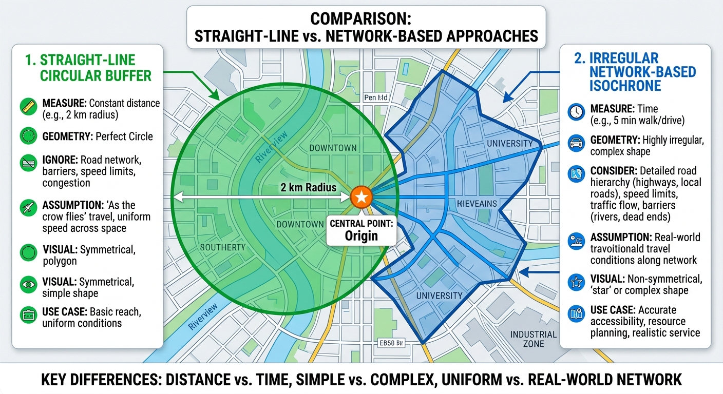
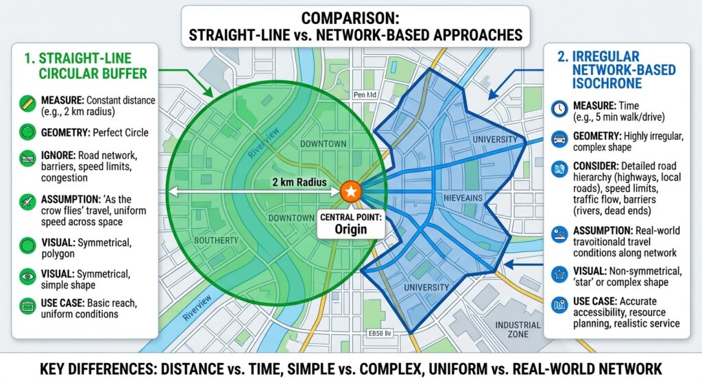
Traditional GIS buffers measure straight-line distance. Isochrones, in contrast, represent areas reachable within a specified travel time or under a specified travel cost using a transportation network.

This distinction is essential for urban accessibility analysis.

What is an isochrone?

An isochrone is a line or polygon connecting locations that can be reached from a starting point within the same travel-time threshold.

For example, a 15-minute driving isochrone around a fire station represents the area that the routing model estimates can be reached within 15 minutes by car, subject to the road network, routing profile, and travel assumptions.

Typical travel-time thresholds include:

5 minutes: Immediate neighbourhood accessibility.
10 minutes: Short urban journeys.
15 minutes: A common illustrative threshold for local service accessibility.
30 minutes: Wider urban or suburban coverage.
60 minutes: Regional access to larger facilities.

These thresholds are examples, not universal planning standards. The appropriate values depend on the service, jurisdiction, population, and policy objective.

Why straight-line buffers can be misleading

Consider a fire station in a city. A 5 km Euclidean buffer includes every location within a 5 km radius of the station, regardless of whether roads or paths actually connect those locations.

An isochrone takes the route network into account.

<box align=”center” gap={2}> <grid columns={2} gap={3}> <grid-item> <AsyncImage query=”urban GIS straight line circular buffer around fire station crossed by river highway network accessibility analysis map” aspectRatio=”4:3″ width=”100%”/> **Euclidean buffer** <text size=”sm”>Shows straight-line proximity, even where barriers force long detours.</text> </grid-item> <grid-item> <AsyncImage query=”GIS urban road network travel time isochrone irregular reachable area polygon around fire station map” aspectRatio=”4:3″ width=”100%”/> **Travel-time isochrone** <text size=”sm”>Shows reachable areas according to the network and routing assumptions.</text> </grid-item> </grid> <text color=”secondary” size=”xs”>Conceptual illustrations; the actual shapes depend on the road network and routing model.</text> </box>

Isochrones are useful for:

Emergency response coverage.
School and hospital accessibility.
Public transport and active-travel planning.
Retail and service catchment analysis.
Identifying underserved urban neighbourhoods.
Evaluating the accessibility impact of road closures or new infrastructure.

This tutorial uses QGIS and the OpenRouteService (ORS) Tools plugin to generate travel-time polygons around facilities. It also explains how to use QGIS’s built-in network analysis and when a Valhalla routing service may be appropriate.

2. Tools Needed

2.1 QGIS

Install QGIS from the official QGIS website. You will use it to prepare facility locations, configure routing, display isochrones, calculate service coverage, and export results.

2.2 OpenRouteService and the ORS Tools plugin

OpenRouteService is a routing service based on OpenStreetMap data. Its APIs support routing, travel-time isochrones, distance matrices, and other network analysis functions.

The ORS Tools plugin connects QGIS to these services and can produce isochrones from one point or from an input layer containing multiple points.

Useful references:

A public ORS account and API key are required for the hosted service. API limits depend on the current service plan, so check the latest restrictions before sending a large batch of requests.

2.3 Other data you may need

For a practical urban accessibility study, prepare:

Dataset	Geometry	Purpose
Fire stations, schools, or clinics	Point	Facility origins
Road network	Line	Optional input for local network analysis
Residential areas or population grid	Polygon or raster	Estimating how many people are served
Administrative boundaries	Polygon	Reporting results by neighbourhood or district
Urban barriers or restricted areas	Polygon	Additional routing constraints, when supported

For the main ORS workflow, you do not need to download and build your own road network because the routing service uses its own network data.

However, local road data remain useful for validating network coverage and identifying missing roads, bridges, or pedestrian connections.

3. Step-by-Step Workflow: Generate Isochrones in QGIS

Step 1: Install the OpenRouteService QGIS plugin

Open QGIS and select:

Plugins → Manage and Install Plugins

In the search box, enter ORS Tools.

Select the plugin maintained by HeiGIT and click Install Plugin. Once installation is complete, look for ORS Tools in the Web menu and in the Processing Toolbox.

The plugin adds tools for routing, isochrones, and other network analyses. Its location and labels can vary slightly with the QGIS and plugin versions.

Step 2: Create an OpenRouteService API key

The hosted routing service requires an API key to authenticate requests.

Open the OpenRouteService website.
Create an account and access the developer dashboard.
Create an API key according to the current account setup.
Copy the key and store it securely.
Return to QGIS and open Web → ORS Tools → Provider Settings or the equivalent configuration option in your installed plugin version.
Select the default OpenRouteService provider and enter the API key.
Save the configuration and confirm that the provider is available.

Do not publish the API key in screenshots, project documentation, public repositories, or shared scripts. Treat it like a password.

If a request fails, check the key, available quota, network connection, service status, and current endpoint restrictions before repeatedly submitting the same request.

Step 3: Prepare the facility origin points

Your origin points represent the facilities from which travel-time accessibility will be measured.

Examples include:

Fire stations.
Schools.
Clinics and hospitals.
Public transport stations.
Community centres.

Load your point layer using Layer → Add Layer → Add Vector Layer.

Check that each feature represents a valid facility and that its coordinates are correct. Remove duplicate records, investigate points located far outside the study area, and confirm that the layer contains a usable identifier such as facility_id or facility_name.

For a facility-coverage study, a useful attribute table might contain:

facility_id	facility_name	type
1	Central Fire Station	Fire station
2	Eastside Fire Station	Fire station
3	Riverside Fire Station	Fire station

These are example records.

The ORS Tools plugin can accept point layers whose coordinates use a different CRS, handling the coordinate conversion required for requests. Nevertheless, verify the input location and CRS before processing. A point with incorrect coordinates cannot be fixed merely by calling a routing API.

Recommended practice: Store your original facility data in GeoPackage and retain a copy before processing.

Step 4: Select the travel mode and time intervals

Open the Processing Toolbox using:

Processing → Toolbox

Search for Isochrones from layer under the ORS Tools group.

Select your facility point layer as the input.

You now need to configure the routing profile and travel-time ranges.

Choosing the travel mode

Common ORS profiles include:

Profile	Typical purpose
`driving-car`	Car-based travel and many road-access studies
`foot-walking`	Pedestrian accessibility
`cycling-regular`	Standard bicycle accessibility

Choose a profile that matches the question you are answering.

For example, a fire-station coverage analysis will normally use a driving profile, while an assessment of walking access to a local clinic should use a pedestrian profile.

The profiles model different access restrictions and routing preferences. A driving isochrone should not be interpreted as pedestrian accessibility, and a general car profile does not automatically represent emergency vehicles with special permissions.

Choosing travel-time intervals

For this tutorial, use three thresholds:

5 minutes.
10 minutes.
15 minutes.

In the ORS Tools interface, configure the maximum time and interval values or individual contour ranges as supported by your version. The plugin commonly provides a maximum range and interval pattern, allowing multiple time thresholds to be requested in one operation.

For example, a maximum time of 15 minutes and an interval of 5 minutes should produce 5-, 10-, and 15-minute contours when using that interface configuration.

Check the units shown in the plugin. The ORS API represents time ranges in seconds, while the plugin interface can present the user with minute-based inputs. Use the units explicitly shown by your installed version rather than copying raw API values into a field expecting minutes.

The public ORS service limits the number of requested locations and intervals per request and also imposes profile-specific maximum ranges. Review the current API restrictions before submitting large jobs.

Step 5: Generate the isochrone polygons

With your facility layer, travel profile, and time thresholds configured, run the Isochrones from layer algorithm.

The tool sends the facility coordinates and requested travel-time ranges to OpenRouteService. It then returns the resulting isochrone features to QGIS.

Save the output to a persistent file such as:

fire_station_isochrones.gpkg

For an analysis of several facilities, inspect the output attributes. Depending on the plugin version and request configuration, fields may include an origin identifier, a location name, a travel-time threshold, or other request-related metadata.

Make sure each contour can be linked to its original facility.

What should you expect?

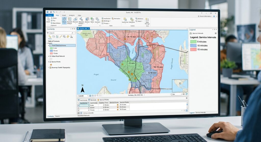
A 5-minute contour will normally be contained within the corresponding 10-minute contour, which is in turn contained within the 15-minute contour for the same origin.

The polygons will often look irregular because roads differ in connectivity and travel cost. High-speed roads can extend a driving catchment in one direction, while rivers, railway lines, disconnected streets, or limited crossings can restrict it elsewhere.

Some providers may return multiple polygon parts for a contour where the reachable network creates disconnected regions. Inspect the geometry rather than assuming every isochrone is a single simple polygon.

Important: These polygons represent modelled network accessibility based on the service’s road data and routing assumptions. They do not necessarily include current traffic, temporary road closures, parking time, emergency dispatch delays, or every local access restriction.

Step 6: Style and compare the overlapping isochrones

Once the polygons have been generated, use symbology to make travel-time thresholds easy to distinguish.

Right-click the output layer and select:

Properties → Symbology

Choose Categorized if your output includes a time-threshold field, such as value, interval, or a plugin-specific travel-time field.

Select the relevant field, classify the categories, and assign distinct colours.

A typical visual hierarchy might use:

A light colour for the 5-minute contour.
A medium shade for the 10-minute contour.
A darker or more saturated shade for the 15-minute contour.

Apply transparency so that roads, neighbourhood boundaries, and facilities remain visible.

If the plugin output does not contain a suitable categorization field, inspect its attribute table and use Processing → Refactor Fields or a field-calculation workflow to create a clear numeric travel-time attribute.

Understand nested polygons

Many isochrone services return cumulative contours. The 15-minute polygon includes locations that are also within 5 and 10 minutes; it is not necessarily a separate 10-to-15-minute band.

This matters for both styling and calculations.

If you want to map exclusive time bands, create ring polygons by subtracting the smaller catchment from the larger one:

0–5 minutes: the 5-minute polygon.
5–10 minutes: the 10-minute polygon minus the 5-minute polygon.
10–15 minutes: the 15-minute polygon minus the 10-minute polygon.

You can use the QGIS Difference tool for these operations. Ensure the polygons correspond to the same facility or correctly combined group of facilities.

For citywide coverage, remember that isochrones from different facilities may overlap. A community served by three facilities must not be counted three times when calculating the unique population covered by the service.

Step 7: Convert the travel-time map into an accessibility analysis

An isochrone map becomes much more useful when you measure the population or services within each travel-time range.

For example, suppose a city wants to determine what proportion of residents can reach at least one fire station within 10 minutes.

Prepare a population grid or residential-area dataset covering the study area.

Option A: Use a population grid

If you have a raster containing population counts per cell, use Processing Toolbox → Zonal Statistics to estimate the population within the isochrone areas.

First, create a single union or dissolved coverage area for the threshold you are evaluating. This ensures that areas covered by overlapping facilities are not counted more than once.

Then:

Dissolve or union the relevant isochrone polygons.
Run Zonal Statistics using the combined coverage polygons and the population raster.
Select the sum statistic if each raster cell stores population counts.
Compare the sum with the total population in the study area.

Use care when the raster stores population density rather than population per cell. Density values must be integrated over the relevant cell or area units instead of being summed blindly.

Option B: Use census or neighbourhood polygons

If population totals are stored in census or neighbourhood polygons, intersect the coverage areas with the population polygons.

If only part of a census polygon lies inside the isochrone, do not automatically count its entire population as accessible. Estimate the population within the intersection using a justified method, such as a population grid or a suitable dasymetric allocation approach.

A simple area-weighted estimate can be used where no better data are available, but it assumes population is distributed evenly within the original polygon. That assumption can be weak in neighbourhoods containing parks, industrial land, large institutions, or uninhabited areas.

Calculate the service-coverage percentage as:

[
\boxed{
\text{Coverage} =
\frac{\text{Population within the catchment}}
{\text{Total population in the study area}}
\times 100
}
]

For example, if 84,000 out of 100,000 residents are estimated to live within a 10-minute driving catchment, the modelled coverage is 84%.

This is an illustrative calculation, not a real assessment.

Step 8: Identify service gaps and export the results

Overlay the combined isochrone coverage with population data and neighbourhood boundaries to identify areas outside the required response-time threshold.

In a fire-response study, you might classify neighbourhoods as:

Within 5 minutes of a station.
5–10 minutes away.
10–15 minutes away.
More than 15 minutes away.

The final category represents potential coverage gaps under the selected routing assumptions. It should not automatically be interpreted as a breach of a formal response standard unless that standard is defined for the service and travel model.

For a clear map, display the facility points above the isochrones, add neighbourhood boundaries, and use a suitable basemap. Add a legend that explains the time thresholds and a note stating the routing profile and data source.

Save the final data using Right-click layer → Export → Save Features As and select GeoPackage, GeoJSON, or another appropriate format. Retain the original facility locations, the isochrone layer, and the derived coverage polygons as separate outputs.

4. Alternative Workflow: QGIS’s Built-In Network Analysis

You can also use QGIS’s native network analysis tools if you have a suitable local road network and want to control travel costs.

Open Processing → Toolbox and search for Service area (from layer).

Configure:

Network layer: Your road network.
Start points: Facility locations.
Path type: Fastest for time-based analysis, or shortest for distance-based analysis.
Travel cost: The cost threshold. For the fastest strategy, QGIS uses seconds.
Speed field: A field containing road speeds in km/h, where available.
Default speed: Used where the selected speed field is missing values.
Direction and topology settings: Set according to the network’s travel restrictions and connectivity.

Run the tool and inspect the output.

A key distinction is that QGIS’s built-in service-area algorithm returns reachable network edges or portions of edges and boundary-node outputs. It does not automatically create the same filled travel-time polygons that an isochrone API usually returns.

To produce polygon coverage from a local network workflow, you need a further polygon-building or surface-modelling step, and should validate how well the resulting polygon represents the network’s reachable area.

The official QGIS Network Analysis documentation describes the service-area tools and their parameters.

5. Using Valhalla as an Alternative Routing Engine

Valhalla is another routing engine with an isochrone service. It can return reachable regions as polygons or contour lines based on a selected travel-costing model.

Its isochrone API supports profiles such as driving (auto), cycling (bicycle), and walking (pedestrian), with configurable contours. Depending on your setup, you can use a hosted Valhalla service or operate an instance yourself, then load the returned GeoJSON into QGIS.

Valhalla is particularly relevant when you need a self-hosted routing workflow or want more control over routing behaviour. However, the available profiles, data coverage, configuration, API limits, and results depend on the particular Valhalla service you use.

See the Valhalla Isochrone API reference for the current request parameters and output options.

6. Common Pitfalls and Quality Checks

Incorrect facility coordinates: A point placed on the wrong street or at the wrong location can create a misleading catchment. Validate facilities against reliable reference data.

Incomplete road networks: Missing bridges, paths, crossings, or local roads can create artificial accessibility gaps. Compare the routing network with local road information.

Wrong travel mode: Walking and driving have different networks, permissions, speeds, and barriers. Always select the profile appropriate to the question.

Assuming constant travel time: A standard routing profile may use modelled speeds rather than real-time traffic. State whether the travel times represent typical modelled conditions, scheduled transit, or observed conditions.

Confusing isochrones with service standards: A 15-minute polygon is a model output. It is not evidence that every trip can be completed within 15 minutes in real conditions.

Double-counting overlapping catchments: Dissolve or union coverage polygons before estimating unique population coverage across multiple facilities.

Ignoring population distribution: Counting everyone in a census polygon when only a small corner falls inside the catchment may overestimate access.

Forgetting API restrictions: Large batches and excessive requests may exceed current limits. Check the provider’s current API policy and split work into reasonable batches.

7. Conclusion

Isochrones provide a more realistic way to assess urban accessibility than straight-line buffers because they account for the transportation network and selected travel mode. They can support emergency-service planning, school accessibility studies, health-facility catchment analysis, and wider urban planning decisions.

The ORS Tools plugin provides a practical route to generating driving, walking, and cycling isochrones directly in QGIS. The native QGIS network analysis tools offer a useful alternative when a local road network and custom speed assumptions are available, while Valhalla provides another API-based routing option.

For a defensible catchment analysis, the essential steps are to validate facility locations, select an appropriate travel profile, generate nested travel-time polygons, account for overlap, and combine the coverage results with population data. Document the routing assumptions and verify the output against local transport conditions before using it for policy or service-planning decisions.