Geographically Weighted Regression (GWR) vs. Multiscale GWR (MGWR): A Practical GIS Guide

 

1. Introduction: Why Spatial Relationships Change Across Geography

When exploring spatial modeling techniques like GWR vs MGWR GIS, Imagine you are studying housing prices across a city. You want to understand how distance to the city centre, household income, and access to public transport influence property prices.

A conventional regression model might estimate that being closer to the city centre is associated with higher prices throughout the study area. But the relationship may not be equally strong everywhere. In the central business district, access to employment may be especially important, whereas in the suburbs, access to schools or transport connections may matter more.

This is an example of spatial non-stationarity: a relationship between variables changes across geographic space.

Two important methods for investigating this phenomenon are Geographically Weighted Regression (GWR) and Multiscale Geographically Weighted Regression (MGWR).

Both extend the basic idea of regression by allowing relationships between variables to vary geographically. Their main difference is the way they define the spatial scale over which each relationship is estimated.

Before comparing them, it helps to understand why ordinary regression may not tell the whole story.

1.1 Why ordinary least squares (OLS) may be insufficient

Ordinary Least Squares (OLS) estimates one global regression equation for the entire dataset. Each explanatory variable has a single coefficient that applies to all observations in the model.

For example:

[
\text{House price} =
\beta_0+\beta_1(\text{Income})+\beta_2(\text{Distance})
]

The coefficients (\beta_1) and (\beta_2) describe the estimated associations between income, distance, and house price under the fitted model.

However, if these relationships vary spatially, a single global coefficient may conceal important local differences. The overall model might fit reasonably well while missing geographic variation that matters for planning or policy.

OLS is not automatically invalid when relationships vary across space. It remains an essential baseline model. The issue is whether a single set of coefficients adequately represents the process being studied.

There is also an important distinction between spatial non-stationarity and spatial autocorrelation in regression residuals. The former concerns changes in relationships across space; the latter concerns spatial patterns remaining in the model errors. GWR and MGWR investigate varying coefficients, but they do not automatically resolve every form of spatial dependence.

For an introduction to the motivation behind GWR, see the foundational paper by Brunsdon, Fotheringham, and Charlton (1996).

2. Understanding Geographically Weighted Regression (GWR)

2.1 What is GWR?

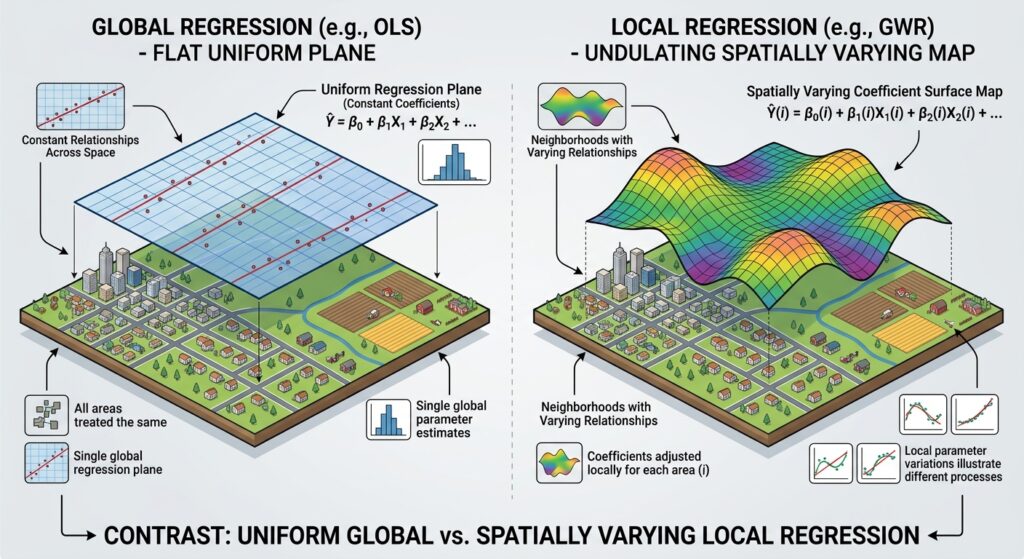
Geographically Weighted Regression estimates a separate local regression model around each observation or selected prediction location.

Instead of using every observation equally to estimate one global equation, GWR gives observations different weights according to their geographic distance from the location being modelled.

Nearby observations generally receive greater weight, while more distant observations receive less weight or, under some weighting schemes, no weight beyond a defined distance.

The model estimates a local coefficient for each explanatory variable at each location. Consequently, the association between a predictor and the dependent variable can differ across the map.

For example, consider a study investigating the relationship between road access and property prices.

• In one part of the city, improved road access may be strongly associated with higher property prices.
• In another part, the estimated relationship may be weak.
• Elsewhere, the relationship may have a different direction after accounting for the other predictors in the model.

GWR helps reveal these local variations.

Key concept: GWR allows the coefficients to vary spatially but ordinarily uses one shared bandwidth for the explanatory variables in a particular model.

2.2 How does a bandwidth work?

A spatial bandwidth determines the geographic extent of the observations influencing a local regression estimate.

Imagine placing a moving window over a city. At each location, the model estimates the local relationship using observations inside that window, with weights determined by a spatial kernel.

A small bandwidth uses a more localized set of observations and can reveal finer spatial differences. A large bandwidth uses a broader set of observations and generally produces smoother coefficient surfaces.

The bandwidth is one of the most important decisions in GWR because it controls the balance between local detail and statistical stability.

2.3 Fixed vs. adaptive bandwidths

GWR commonly offers two approaches to defining the neighbourhood.

Fixed bandwidth

A fixed bandwidth uses the same geographic distance at every location.

For example, the model might use observations within a 10-kilometre radius of each target location, subject to the chosen kernel.

This can be useful when a consistent geographic interaction distance is meaningful and the observations are reasonably evenly distributed.

However, a fixed distance may include many observations in a dense urban centre and very few in a sparsely populated rural area.

Adaptive bandwidth

An adaptive bandwidth uses a specified number of nearest neighbours. The geographic radius expands or contracts according to the density of observations.

For example, the model might use the 80 nearest observations for each local regression. The actual radius may be small in a dense city centre and much larger in the surrounding countryside.

This is useful when observations are unevenly distributed.

Feature	Fixed bandwidth	Adaptive bandwidth
What remains constant?	Geographic distance	Number of neighbours
Neighbourhood size	Same radius throughout	Radius varies by location
Best suited to	Fairly even spatial sampling or a meaningful fixed distance	Unevenly distributed observations
Main risk	Too few observations in sparse areas	Very different geographic scales across locations

Neither method is universally superior. Choose the approach based on the spatial distribution of your data and the process you are investigating.

GWR implementations often select the bandwidth using criteria such as the corrected Akaike Information Criterion (AICc) or cross-validation (CV). These methods help identify a bandwidth that balances model fit with complexity or predictive performance. See the ArcGIS Pro GWR documentation.

2.4 Understanding local coefficients

One of the most useful GWR outputs is the set of local regression coefficients.

Suppose you model house prices using median income and distance from the city centre. GWR estimates a local income coefficient and a local distance coefficient for each location.

Imagine the estimated income coefficient is larger in one neighbourhood than another. This suggests that the association between income and house prices is stronger in the first location, conditional on the other variables and the model specification.

When interpreting local coefficients, consider:

• Sign: A positive coefficient indicates a positive conditional association; a negative coefficient indicates a negative conditional association.
• Magnitude: The size of the coefficient describes the strength of the estimated relationship in the variables’ units.
• Spatial variation: Changes across locations may indicate non-stationarity, although they may also reflect sampling variation or modelling problems.
• Uncertainty: Inspect local standard errors and relevant inference results, rather than assuming every visible coefficient difference is statistically meaningful.

Do not interpret a positive local coefficient as proof that one variable causes another. GWR is a regression method, and causal claims require an appropriate research design and additional evidence.

2.5 Understanding local R-squared

GWR may provide a local R-squared value for each location. This describes how well the local regression fits the observations used in that location’s weighted model.

For example:

• A local R-squared of 0.80 suggests that the fitted local model explains a substantial proportion of the weighted variation in the dependent variable.
• A local R-squared of 0.25 suggests that the local model explains a smaller proportion of that variation.

These values are illustrative. Local R-squared is a measure of fit, not proof that the model is scientifically correct or that its coefficients are significant.

Mapping local R-squared can help identify where the model performs relatively well and where it struggles. Low values might indicate important omitted variables, weak relationships, noisy measurements, or an unsuitable model specification.

High local R-squared values must also be interpreted with care because a very small bandwidth can produce unstable local estimates and overly optimistic fit.

3. The Evolution to Multiscale Geographically Weighted Regression (MGWR)

3.1 Why was MGWR developed?

Standard GWR assumes that all explanatory variables operate at the same spatial scale within the model. In practice, this may be restrictive.

Consider a study of house prices with three explanatory variables:

• Household income.
• Distance to the city centre.
• Access to local parks.

The influence of household income may vary gradually across a large region. Distance to the city centre may matter at an intermediate scale, while access to parks may be most strongly related to prices within relatively small neighbourhoods.

If standard GWR uses one bandwidth for all three predictors, it cannot independently match the spatial scale of each relationship.

MGWR addresses this limitation by estimating a separate bandwidth for each explanatory variable.

This approach was developed in the multiscale GWR literature, including the work of Fotheringham, Yang, and Kang (2017).

3.2 How does MGWR work?

Multiscale Geographically Weighted Regression (MGWR) extends GWR by allowing each explanatory variable to have its own spatial bandwidth.

Instead of assuming one shared local neighbourhood, MGWR estimates different neighbourhood scales for different coefficients.

Conceptually, a model might identify:

Explanatory variable	Illustrative estimated scale	Possible interpretation
Regional accessibility	180 neighbours	The relationship varies gradually across a broad area
Distance to city centre	95 neighbours	The relationship varies at an intermediate scale
Local park access	35 neighbours	The relationship varies more locally

These neighbour counts are hypothetical, not recommended settings. Their geographic meaning depends on the distribution of observations and the bandwidth method used.

A larger estimated bandwidth generally indicates a smoother, broader-scale coefficient surface. A smaller bandwidth indicates that the coefficient is estimated using a more localized neighbourhood and can vary more rapidly across space.

However, a bandwidth does not automatically identify the real-world causal range of a process. It is the scale selected by the model for estimating a relationship, under the chosen data, variables, kernel, and selection method.

3.3 Why different variables need different scales

Spatial processes do not all operate at the same geographic scale.

A regional labour market may influence income across a wide area. Access to a local primary school may matter within a smaller catchment. Neighbourhood green space might influence housing prices differently over relatively short distances.

MGWR can represent these different scales within one model, rather than requiring all coefficients to use the same neighbourhood.

This can help answer questions such as:

• Does the influence of transport access change locally or regionally?
• Is the relationship between income and housing prices spatially smooth?
• Do environmental variables exhibit broader or more localized associations with the outcome?
• Does a shared bandwidth oversmooth some relationships while undersmoothing others?

MGWR does not guarantee a better scientific model simply because it is more flexible. Its results still depend on appropriate data, reasonable predictors, and well-diagnosed statistical assumptions.

3.4 Understanding MGWR bandwidth outputs

MGWR typically produces a selected bandwidth for each explanatory variable, including the intercept in implementations that estimate a local intercept.

These bandwidths allow the analyst to compare the spatial scales represented by different coefficient surfaces.

When interpreting them:

• A broad bandwidth suggests that the estimated coefficient changes relatively smoothly across the study area.
• A narrower bandwidth suggests that more localized variation is needed to fit the relationship.
• Similar bandwidths across variables suggest that the data do not require dramatically different scales for those relationships under the chosen model.
• A bandwidth approaching the global sample size may suggest that a coefficient is effectively operating at a broad or nearly global scale.

The final conclusion should be based on the bandwidth estimates alongside model diagnostics, not on the bandwidth values alone.

4. GWR vs. MGWR: Direct Comparison

Feature	OLS	GWR	MGWR
Model type	Global regression	Local regression	Local regression with variable-specific scales
Coefficients	One coefficient per predictor for the whole dataset	Coefficients vary by location	Coefficients vary by location and use separate bandwidths
Bandwidth assumption	None	One shared bandwidth for local predictors	A separate bandwidth for each predictor
Spatial non-stationarity	Not directly represented in coefficients	Can represent spatially varying coefficients	Can represent spatially varying coefficients at different scales
Scale sensitivity	No local bandwidth	Sensitive to the chosen bandwidth	Sensitive to multiple selected bandwidths
Complexity	Lowest	Moderate	Highest of the three
Computational requirements	Usually lowest	Higher because many local models are estimated	Often higher than GWR because multiple bandwidths must be estimated
Interpretation	Simple global relationships	Local relationships under a common spatial scale	Local relationships at potentially different spatial scales
Typical diagnostics	R-squared, adjusted R-squared, residuals, coefficient tests	Global and local fit statistics, residuals, local coefficients	Model fit, variable-specific bandwidths, local coefficients and uncertainty
Best use case	Baseline modelling with broadly stationary relationships	Exploring local relationships when a shared scale is reasonable	Exploring processes whose predictor relationships vary at different spatial scales

Which model captures the most detail?

MGWR is more flexible than standard GWR because it permits different spatial scales. However, more flexibility does not automatically mean a more reliable explanation.

A complex model may be sensitive to the selected variables, local multicollinearity, outliers, and sample distribution. This is why OLS remains important as a baseline, GWR is useful for examining local relationships, and MGWR is valuable when the research question specifically concerns varying spatial scales.

5. Practical Example: Modelling House Prices

Suppose a researcher wants to understand house prices across a metropolitan region. The dependent variable is house price, and the explanatory variables are household income, distance to the city centre, and proximity to parks.

The objective is to understand how these variables relate to house prices and whether those relationships vary geographically.

Step 1: Prepare the data

• Collect property prices or suitable area-level housing-price data.
• Obtain income, park-access, and distance-to-centre variables.
• Check missing records and outliers.
• Ensure that all geographic data use suitable coordinate systems.
• Investigate whether the predictors are strongly correlated.
• Confirm that the outcome and predictor measurements are comparable across space.

Step 2: Fit an OLS baseline model

Estimate a global relationship between house prices and the selected predictors.

Review residuals, goodness of fit, predictor relationships, and possible spatial patterns in the residuals.

If the global coefficients provide a reasonable account of the process and there is little evidence of meaningful coefficient non-stationarity, a global model may be sufficient.

If relationships appear to vary across the study area, investigate whether a local model is justified.

Step 3: Fit GWR

Estimate a GWR model with an appropriate bandwidth selection procedure.

Map the coefficient for each predictor and inspect local model fit. For example, the income coefficient might be stronger in the inner city and weaker in some outer suburbs.

Check whether the observed coefficient variation is stable and interpretable, rather than relying solely on the visual pattern of the coefficient map.

Step 4: Fit MGWR if different scales are plausible

If the research hypothesis suggests that different explanatory variables operate at different geographic scales, fit MGWR.

Compare the selected bandwidths:

• Income may use a relatively broad bandwidth.
• Distance to the city centre may use an intermediate bandwidth.
• Access to parks may use a narrower bandwidth.

These results may suggest that different mechanisms are associated with house prices at different spatial scales. They do not, by themselves, prove the mechanisms are causal.

Step 5: Compare and validate the models

Use relevant diagnostics to compare OLS, GWR, and MGWR:

• AICc: Lower values generally indicate a preferable balance of model fit and complexity among comparable fitted models.
• Adjusted R-squared: Helps summarize fit while accounting for model complexity, although interpretation differs across model frameworks.
• Residual analysis: Checks whether the unexplained errors have systematic patterns or problematic distributions.
• Cross-validation: Evaluates predictive performance using observations not used in each fit, where the design is appropriate.
• Coefficient stability: Checks whether local coefficients change dramatically under reasonable modelling choices.
• Collinearity diagnostics: Identifies predictors that may be too strongly related to distinguish their local effects reliably.

Do not select MGWR solely because it produces visually interesting maps. Prefer the model that best addresses the research question and performs adequately under the relevant diagnostics.

6. Practical Workflow in ArcGIS Pro and Python

6.1 ArcGIS Pro

ArcGIS Pro provides separate tools for GWR and MGWR.

For GWR:

• Open Analysis → Tools.
• Search for Geographically Weighted Regression.
• Select the dependent variable and explanatory variables.
• Choose an appropriate neighborhood method, fixed or adaptive kernel, and bandwidth-selection method.
• Define output features and inspect the diagnostic results.

For MGWR:

• Open Analysis → Tools.
• Search for Multiscale Geographically Weighted Regression.
• Select the dependent variable and explanatory variables.
• Configure neighbourhood selection and kernel settings.
• Review the variable-specific bandwidth outputs and diagnostics.

Consult the current GWR tool reference and MGWR tool reference for supported parameters and model requirements.

Important model-family distinction: Available regression families differ between tools and software implementations. ArcGIS Pro’s current MGWR tool is intended for continuous dependent variables; it should not be used directly with binary outcomes or raw count outcomes. GWR implementations may support additional model families, such as Poisson or logistic regression. Choose the model family appropriate for the response variable rather than treating every outcome as ordinary continuous data.

6.2 Python with PySAL’s mgwr package

The open-source mgwr package supports bandwidth selection and estimation for GWR and MGWR. It is useful when you want a reproducible Python workflow and wish to combine spatial modelling with GeoPandas and pandas.

Official resources include:

• MGWR documentation
• Bandwidth selection API
• GWR API

A practical Python workflow generally involves:

1. Load and inspect the spatial dataset.
2. Select the response and predictor variables.
3. Prepare coordinates in an appropriate coordinate system.
4. Check missing values, outliers, and predictor correlations.
5. Standardize variables where appropriate and document the interpretation.
6. Select a bandwidth for GWR or variable-specific bandwidths for MGWR.
7. Fit the model and inspect diagnostics.
8. Join estimated coefficients and fitted values back to the spatial data.
9. Map coefficient surfaces, residuals, and local fit measures.
10. Save the outputs and document the model assumptions.

The Python package’s MGWR implementation is based on Gaussian regression, so confirm that the chosen implementation supports the outcome type and assumptions of your project before fitting the model.

7. When Should You Choose OLS, GWR, or MGWR?

Use the following decision guide when planning a thesis project.

Choose OLS when:

• You need a simple baseline model.
• A single global relationship is appropriate to the research question.
• Your diagnostics do not show compelling evidence that local coefficients are necessary.
• Interpretability and parsimony are priorities.

Choose GWR when:

• You have a defensible reason to expect spatial non-stationarity.
• Local coefficient maps directly address your research question.
• A shared spatial bandwidth is reasonable for the variables being studied.
• Your dataset is sufficiently large and spatially informative for local estimation.

Choose MGWR when:

• You expect different predictors to operate at different geographic scales.
• GWR appears to impose an overly restrictive common bandwidth.
• You have enough observations to estimate multiple bandwidths reliably.
• The additional modelling complexity is justified by the scientific question.

Questions to ask before choosing a model

• Is the dependent variable continuous, binary, or a count?
• Are the observations geographically well distributed?
• Is there sufficient sample size for local estimation?
• Are explanatory variables strongly correlated globally or within local neighborhoods?
• Is coefficient variation substantively meaningful, or could it be caused by sampling noise?
• Does the model improve on a reasonable global baseline?
• Have you examined residual patterns and predictive validation?

No regression technique should be selected simply because it is more advanced. The method should match the data, statistical assumptions, and research objective.

8. Important Limitations and Reporting Advice

GWR and MGWR are useful tools, but they introduce challenges that students should acknowledge.

Local multicollinearity: Predictors that are closely related can make local coefficients unstable or difficult to distinguish. Examine global and local collinearity diagnostics where available.

Bandwidth sensitivity: Coefficient surfaces and local fit can change depending on bandwidth choices. Use a defensible selection criterion and document the chosen scale.

Multiple testing: If you map local coefficient significance at hundreds of locations, some apparently significant results may arise by chance. Consider suitable inferential procedures and avoid treating every local p-value as definitive.

Spatial autocorrelation: Check model residuals for spatial patterns. GWR and MGWR model spatially varying coefficients; they do not guarantee that residual spatial dependence has been eliminated.

Interpretation: A local coefficient shows a conditional association under the fitted model, not proof of a causal mechanism.

For an academic report, document the dependent variable, predictors, sample size, coordinate system, bandwidth type and selection method, model diagnostics, residual checks, and limitations. When comparing models, explain why the chosen model addresses the research question more effectively than the alternatives.

9. Conclusion: The Right Regression Model Depends on the Question

OLS, GWR, and MGWR each serve a distinct purpose in spatial modelling.

OLS provides a global baseline with one set of coefficients. GWR allows the coefficients to vary across space but assumes a common bandwidth for the explanatory variables. MGWR extends this approach by estimating different bandwidths for different variables, allowing relationships to vary at multiple spatial scales.

For students, a defensible research workflow begins with a well-specified global model, investigates evidence of spatial non-stationarity, and then considers GWR or MGWR when the data and scientific question support their use.

The central lesson is that the most sophisticated model is not always the best one. Select the method that provides a clear, statistically defensible answer to your research question, and support your interpretation with appropriate diagnostics and validation.

Use OLS to establish the baseline, GWR to investigate local variation, and MGWR to examine whether different relationships operate at different spatial scales.