Table of Contents

Georeferencing Scanned Paper Maps & Imagery: 5 Steps to Match Real-World Coordinates

1. Introduction: What Is Georeferencing?

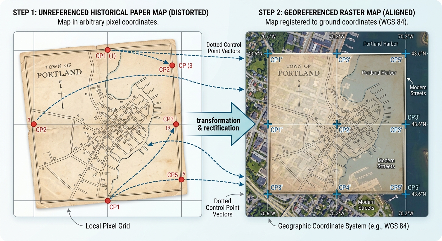
When mastering Georeferencing Scanned Maps QGIS ArcGIS Pro workflows, Imagine you find a scanned paper map showing roads, settlements, rivers, and administrative boundaries from 1960. The map is clear, but when you load the image into QGIS or ArcGIS Pro, it appears in the wrong location or has no geographic coordinates at all.

You cannot reliably overlay it with modern satellite imagery, compare historical boundaries, or measure distances until its pixels are associated with real-world locations.

This process is called georeferencing.

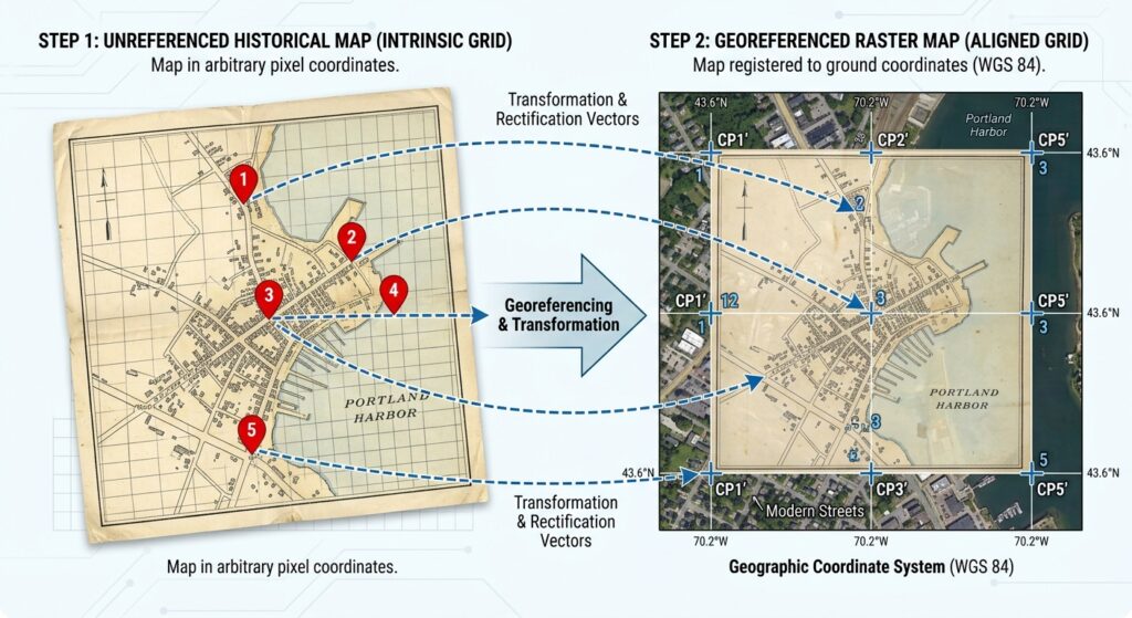
Georeferencing aligns an image or map with a known geographic coordinate system by matching identifiable locations on the source image to their corresponding positions in spatially referenced data. These matching locations are called Ground Control Points (GCPs).

Common applications include:

Historical GIS: Comparing old land-use maps with modern satellite imagery to investigate urban expansion.
Cartography: Aligning scanned topographic maps with modern vector boundaries.
Remote sensing: Registering imagery to a reference dataset when its existing spatial alignment is insufficient.
Environmental research: Comparing historical shorelines, wetlands, forests, and river courses with present-day conditions.

Two widely used applications for this work are QGIS and ArcGIS Pro. Both support control points, transformation algorithms, error assessment, and exporting georeferenced rasters. See the QGIS Georeferencer documentation and ArcGIS Pro georeferencing overview.

This tutorial follows five steps:

Prepare a suitable reference dataset.
Add Ground Control Points.
Select a transformation algorithm.
Evaluate and minimize RMS error.
Rectify and export the georeferenced image.

2. Step 1: Prepare Your Target Base Dataset

Before georeferencing, identify the dataset that will provide the correct geographic reference for your scanned map.

This reference is called the target dataset. It may be a georeferenced satellite image, a reliable basemap, or a vector dataset containing identifiable geographic features.

2.1 Choose a suitable reference layer

Good reference layers include:

A georeferenced topographic map covering the same area.
A reliable orthorectified aerial image or satellite image.
A vector layer containing established roads, intersections, or administrative boundaries.
Surveyed control points with known coordinates.

For a historical map, your reference should contain features that can be confidently matched between the historical and modern datasets.

For example, if you are georeferencing a scanned map of Nairobi from the 1960s, you could use stable road junctions or long-established railway crossings that remain identifiable in an appropriate reference layer.

Avoid assuming that every feature visible on an old map still occupies the same position today. Roads may have been rerouted, rivers may have changed course, and shorelines may have migrated.

2.2 Load the reference data into QGIS

Open QGIS and create a new project or open your existing project.
Add the georeferenced reference layer using Layer → Add Layer or the appropriate browser panel.
Confirm that the reference layer appears in the correct geographic location.
Right-click the layer and open Properties to inspect its coordinate reference system (CRS).
Confirm that the CRS is appropriate for your study area and measurement objectives.

If your reference layer has an incorrect or unknown CRS, resolve that problem before collecting control points. Georeferencing will not fix an incorrectly defined reference dataset.

2.3 Load the reference data into ArcGIS Pro

Open your project and add the reference raster or vector layer to the map.
Confirm that the map displays the reference layer in the correct location.
Check the layer’s spatial reference and verify that its coordinates are trustworthy.
Ensure the reference features you plan to use can be identified clearly.

ArcGIS Pro uses the reference layer to establish the target coordinates for your control points.

2.4 Prepare the scanned map

Before collecting control points, check that your scanned image is suitable for georeferencing.

Ensure the entire map area is visible and legible.
Identify any map border, legend, scale bar, neatline, or marginal information that should not be included in your final geographic raster.
Check whether the map has a printed coordinate grid or graticule.
Look for signs of scanning distortion, folded paper, stretching, or rotation.

If the map contains substantial blank margins, you may crop them before georeferencing. However, preserve the original scan because it may contain useful information for historical documentation.

Cartographic advice: A scanned map’s printed CRS and projection information can be extremely valuable. If the original map has a coordinate grid, projection name, datum, and grid coordinates, use those details to establish the target reference rather than relying exclusively on visual matching.

3. Step 2: Add Ground Control Points (GCPs)

Ground Control Points are the foundation of georeferencing. Each point links a recognizable location on the source image to the same location in a reference dataset or to known real-world coordinates.

For example, a clearly identifiable road intersection on a historical map may correspond to the same intersection in a modern reference layer.

The georeferencing software uses these matched locations to estimate the transformation needed to position the entire image. Esri’s georeferencing overview explains this control-point workflow.

3.1 What makes a good control point?

A suitable GCP should be easy to identify accurately on both the source image and the reference data.

Good candidates include:

Road intersections that have remained in the same location.
Corners of long-established buildings or structures.
Bridge crossings that have not moved.
Established survey markers or coordinate-grid intersections.
Distinctive and stable land features that can be matched precisely.

Less suitable candidates include:

Tree canopies or isolated vegetation patches that may have changed.
Broad, indistinct coastline sections.
River bends that have migrated over time.
Blurred features or poorly defined map symbols.
Features whose positions have changed between the historical map and the modern reference.

For historical GIS, the key question is not simply whether a location is visible. It is whether the same physical location can be identified reliably across both sources.

3.2 Distribute points across the map

Control-point placement strongly influences the transformation.

A useful arrangement includes points near the corners, along the edges, and throughout the interior of the map.

A good distribution helps constrain the transformation across the full image, rather than fitting only a small central section.

Avoid placing all GCPs in one corner or along a single road. Poorly distributed points may produce an image that aligns well in one area but is distorted elsewhere.

3.3 Add GCPs in QGIS

Open Layer → Georeferencer. Menu placement can vary by QGIS version.
In the Georeferencer window, open the scanned raster.
Use Add Point to select a recognizable location on the scanned image.
Choose From Map Canvas to identify its matching position on the reference layer, or enter verified X and Y coordinates manually.
Repeat the process for additional locations distributed across the image.
Review the control-point table and correct any misplaced points.
Save the GCP points so they can be reused or reviewed later.

QGIS can use an existing spatially referenced layer in the main map canvas to supply the target coordinates. It also supports entering known coordinates directly. See the QGIS control-point instructions.

3.4 Add GCPs in ArcGIS Pro

Add the scanned raster to the map.
Select the raster in the Contents pane.
Open the Imagery tab and click Georeference.
On the Georeference tab, select Add Control Points.
Click a recognizable location on the source raster.
Click its corresponding location on the reference layer.
Repeat for additional points and inspect the Control Point Table.

In ArcGIS Pro, the point pair connects a source-raster location to a target-map location. Check that you select the correct location on each side of every pair.

3.5 How many GCPs do you need?

The minimum number depends on the transformation algorithm.

Transformation	Minimum GCPs	Practical recommendation
Linear in QGIS	2	For basic positioning and uniform scaling
Helmert in QGIS	2	For translation, rotation, and uniform scaling
First-order polynomial	3	Use additional well-distributed points
Second-order polynomial	6	Use additional points across the map
Third-order polynomial	10	Use more well-distributed points and carefully inspect distortion
Projective	4	Useful for perspective distortion
Thin Plate Spline (TPS)	Technically 10 in QGIS	Usually requires more points for a stable result

These are algorithmic minimums, not recommendations to use only that many points. The transformation options and minimums are documented in the QGIS Georeferencer guide and ArcGIS Pro georeferencing tools.

A first-order polynomial typically needs at least three non-collinear control points. Higher-order transformations require more points because they estimate more complex relationships.

For an ordinary scanned map, begin with a first-order transformation and several well-distributed GCPs. Only move to a more complex model when the map’s distortion justifies it.

4. Step 3: Select the Right Transformation Algorithm

A transformation algorithm defines how source-image coordinates are converted into target-map coordinates.

The right choice depends on the map’s condition, the source of distortion, the number and quality of GCPs, and the intended use of the output.

4.1 Linear and Helmert transformations

In QGIS, the Linear transformation creates a world file for positioning and uniformly scaling an image without actually resampling its raster pixels. It does not provide the same flexibility as a full affine transformation.

The Helmert transformation adds rotation while preserving the image’s shape through uniform scaling. It is useful when a good-quality raster is simply rotated or offset.

Choose these options when the source map is already geometrically sound and you mainly need to position or orient it.

4.2 First-order polynomial: Affine transformation

A first-order polynomial transformation, also called an affine transformation, can translate, rotate, scale, and shear the image.

It is often a good starting point for georeferencing flat scanned paper maps that have uniform scanning distortion but do not require substantial local warping.

Use it when:

The scanned map is in reasonably good condition.
Straight map lines should remain straight.
Distortion is relatively uniform across the image.
You want a relatively simple and stable transformation.

A first-order affine transformation may introduce small residual errors at individual GCPs when more than the minimum number of points is used. That is normal because the model finds an overall least-squares fit rather than forcing every control point to match exactly.

4.3 Second- and third-order polynomial transformations

Higher-order polynomial models allow more complex, smoothly varying distortions.

A second-order polynomial can model more curvature than an affine transformation. A third-order polynomial is more flexible still, but it also requires more control points and can distort areas away from the GCPs.

Algorithm	Typical use	Main caution
First-order polynomial	General scanned-map alignment	Cannot model substantial curved distortion
Second-order polynomial	Moderate systematic warping	Can distort edges if the GCP arrangement is weak
Third-order polynomial	More complex map distortion	Greater risk of overfitting and edge instability

Higher-order transformations should not be selected simply because they produce a smaller RMS error. They can fit the available points more closely while producing unrealistic geometry between points or near the image edges.

4.4 Thin Plate Spline (Spline)

The Thin Plate Spline transformation, often described as rubber sheeting, aims to fit the control points precisely while deforming the image locally.

It can be useful for:

Damaged or stretched historical maps.
Scans with local paper deformation.
Maps with irregular distortions that cannot be represented adequately by a simple polynomial.

However, the image may be distorted considerably between GCPs, particularly where point placement is inaccurate.

TPS is not automatically the best choice for historical maps. If the purpose is to compare distances, areas, or boundary positions, a model that fits the points exactly may still produce an unreliable result between them.

4.5 Projective transformation

A projective transformation is particularly useful when georeferencing photographs of maps taken at an angle rather than flat scans.

It accounts for perspective effects, such as the apparent convergence of lines that were parallel on the original map.

Use it for suitable oblique photographs or imagery affected by perspective. A flat, well-scanned map usually does not need this transformation.

Choosing in the software

In QGIS:

Open Transformation Settings in the Georeferencer.
Choose the transformation type.
Set the target CRS.
Choose an appropriate resampling method.
Specify the output raster path.

In ArcGIS Pro:

Open the Georeference tab.
Select Transformation.
Choose the appropriate transformation.
Review the control-point residuals and alignment.
Repeat with a different transformation only when the evidence supports the change.

The transformation names and available settings differ between QGIS and ArcGIS Pro. In particular, QGIS Linear and ArcGIS Pro’s first-order polynomial should not be treated as identical methods.

5. Step 4: Evaluate and Minimize RMS Error

Once the GCPs and transformation are configured, evaluate how well the model aligns the scanned map to the reference data.

One of the most commonly reported measures is the Root Mean Square (RMS) error.

RMS error summarizes the differences between the target coordinates and the coordinates predicted by the transformation for the control points.

In simple terms, it helps you understand how closely the fitted transformation matches the GCPs used in the adjustment.

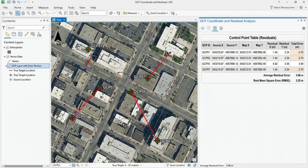
5.1 Understand residual error

A residual is the difference between the target location of a GCP and the location predicted by the transformation.

Suppose a road intersection on the source image is matched to a known location on the reference map. After calculating the transformation, the software estimates where that intersection should fall in the output raster.

The difference between the known target location and the predicted location is the residual.

If the software reports residuals in map units, they may be expressed in metres or feet. If reported in pixels, they express the discrepancy relative to the raster’s pixel coordinates.

The exact summary and units depend on the application and its display settings. In QGIS, consult the GCP table and, if generated, the PDF report. In ArcGIS Pro, inspect the Control Point Table and its error information.

5.2 What counts as a good RMS error?

There is no single RMS threshold that is appropriate for every project.

An error of 5 metres may be acceptable for a coarse historical regional map but unsuitable for a high-accuracy engineering survey. A scanned map’s original scale, printing distortion, line thickness, source-data accuracy, and pixel size all influence the achievable alignment.

Use the following as a conceptual guide, not a universal grading scale.

RMS error	General interpretation
Very low relative to your accuracy requirement	The transformation fits the selected GCPs closely
Moderate relative to your requirement	Review individual residuals and local alignment carefully
High relative to your requirement	Investigate incorrect control points, unsuitable transformations, or incompatible reference data

A small RMS error does not guarantee that the entire output raster is geographically accurate. It summarizes the fit to the selected control points and does not automatically measure the accuracy of every pixel.

5.3 How to reduce RMS error properly

Use these checks in order:

Verify the point pairs. Confirm that each source point corresponds to the correct target point.
Check the reference CRS. Make sure the target coordinates come from the intended coordinate system.
Review the largest residuals. Investigate any GCP whose error is substantially higher than the others.
Improve the distribution. Add reliable GCPs near underrepresented edges and interior areas.
Test an appropriate transformation. If the distortion is not uniform, a more flexible model may be justified.
Inspect the whole image. Check whether roads, boundaries, and recognizable features align beyond the points used to fit the model.

Do not delete a GCP merely because it increases the RMS error. First determine whether the point is inaccurate or whether it reveals a genuine weakness in the transformation.

5.4 Avoid overfitting

A high-order polynomial or TPS model may match the control points very closely, even when the output between those points is distorted.

To reduce this risk, reserve some reliable, well-distributed points as independent check points where possible. Do not use those points to fit the transformation; instead, use them to assess how well the finished map aligns at locations excluded from the adjustment.

This distinction is especially important for historical maps, where paper shrinkage and changes in physical features can make perfect alignment impossible.

If your thesis requires quantitative positional accuracy, document the point-selection method, transformation, residuals, independent check-point results, and source-map scale.

6. Step 5: Rectify and Export the GeoTIFF

Once the transformation is satisfactory, create the georeferenced output.

Rectification means resampling the source raster into a new grid that aligns with the target coordinate system. This differs from simply storing georeferencing information alongside the original, unchanged pixels.

6.1 Export a GeoTIFF in QGIS

Open the Georeferencer’s Transformation Settings.
Select the appropriate target CRS.
Enter an output filename ending in .tif.
Choose a suitable resampling method.
Set the output resolution if needed.
Enable saving GCP points if you want to preserve the control-point information.
Click Start Georeferencing.
Load the output GeoTIFF into the QGIS map canvas.

For transformed outputs, QGIS can create a new georeferenced raster. Linear and Helmert transformations can instead create a world file without resampling the pixels. If your project requires a rectified GeoTIFF, make sure you choose a transformation and output workflow that actually creates the raster.

See the QGIS transformation and output settings.

6.2 Choose a resampling method

Resampling determines how raster pixel values are calculated when the image is mapped onto the new grid.

Method	Best suited to	Key consideration
Nearest neighbour	Categorical or classified raster values	Preserves original pixel values
Bilinear	Continuous imagery	Produces smoother values
Cubic	Continuous imagery needing smoother appearance	Can introduce new pixel values

For a scanned historical map, the best method depends on the map’s content. If the image contains discrete classes or carefully preserved pixel values, nearest neighbour may be appropriate. If visual smoothness is more important, bilinear or cubic interpolation may be suitable.

6.3 Save the result in ArcGIS Pro

On the Georeference tab, review the control points and transformation.
Use Save if you want to save the georeferencing information with the existing raster and its supporting files.
Use Save As New if you need a separate output raster with the georeferencing result.
If your workflow requires a specific GeoTIFF output, confirm the output format and location through the available save options or a suitable raster export workflow.
Export the control-point information when you need a record of the transformation.

ArcGIS Pro distinguishes between saving georeferencing information and creating a new raster dataset. Choose the approach appropriate to your output requirements. See the ArcGIS Pro georeferencing tools.

6.4 Verify the output

After exporting, do not assume the job is complete.

Overlay the GeoTIFF on the target reference layer.
Check road intersections, map boundaries, waterways, or other recognizable locations.
Inspect areas between the GCPs, not just the control-point locations.
Confirm the output CRS and geographic extent.
Record the transformation type, residual results, and any limitations.

For historical analysis, remember that an old map may have been produced using a different survey method, projection, or datum. Some positional differences may reflect the source map itself rather than a failure of your georeferencing workflow.

7. Troubleshooting: When Your Map Stretches, Warps, or Flips

Problem 1: The raster stretches or becomes distorted

Possible causes: Poorly placed control points, inadequate point distribution, an unsuitable transformation, or real distortion in the scanned paper map.

What to do:

Review the GCP table and check for misplaced points.
Remove or correct demonstrably inaccurate points.
Add trustworthy control points in regions that lack coverage.
Return to a simpler transformation if the high-order model introduces unrealistic curvature.
Inspect the scan for damage or uneven paper deformation.

Avoid using increasingly complex transformations solely to improve the RMS value. The output should be geographically plausible, not merely mathematically fitted to the GCPs.

Problem 2: The map flips upside down or appears on the wrong side of the world

Possible causes: Reversed coordinates, incorrect target coordinates, wrong CRS selection, or incorrect point pairing.

What to do:

Confirm that the source point and corresponding target point have not been confused.
Verify that longitude and latitude or projected X and Y coordinates are in the expected order.
Check that you selected the correct target CRS.
Review the GCPs for swapped or incorrectly entered coordinate values.
Recheck the transformation after correcting the control points.

For QGIS, the coordinate values entered for a point must match the CRS declared for those coordinates. In ArcGIS Pro, ensure that each source-raster click is followed by the corresponding target-map location.

Problem 3: The RMS error is low, but the map looks wrong

Possible causes: Too few control points, a poorly distributed GCP set, an overly flexible transformation, or mismatches between old and modern geographic features.

What to do:

Examine individual residuals instead of relying on the summary RMS.
Check the alignment of features between control points.
Use independent check points where possible.
Compare the output against a second trustworthy reference source if one is available.
Consider whether historical roads, rivers, or boundaries have genuinely changed.

A low RMS value can indicate that the model fits the selected GCPs well without proving that the whole map has accurate geographic positioning.

Problem 4: The GeoTIFF does not align when opened in another GIS application

Possible causes: Incorrect output CRS, missing georeferencing information, or an output saved as a different file type than intended.

What to do:

Inspect the output’s CRS and extent.
Confirm that you exported a georeferenced raster, not just an unreferenced image.
If using a world file, ensure it remains with the associated image and that the GIS application recognizes it.
Re-export if necessary, using a suitable format and explicitly defined CRS.

8. Summary: Building a Reliable Georeferencing Workflow

Georeferencing allows scanned paper maps, historical imagery, and other unreferenced images to be used alongside modern spatial datasets.

The five steps are:

Prepare the target dataset: Use a reliable reference layer with a known coordinate system.
Add control points: Match stable, identifiable locations and distribute them throughout the image.
Select a transformation: Start with the simplest model appropriate to the source distortion.
Evaluate RMS error: Review residuals and test independent locations rather than relying only on one number.
Export and validate: Create a suitable georeferenced output and inspect its alignment throughout the image.

For university assignments, the most important skills are choosing reliable Ground Control Points, understanding the assumptions behind transformation algorithms, and interpreting RMS error in the context of the source map’s accuracy.

A successful georeferencing workflow does not simply make an image fit a basemap. It establishes a defensible relationship between the image and real-world coordinates, documents its limitations, and produces a spatial dataset that can be used responsibly in further analysis.