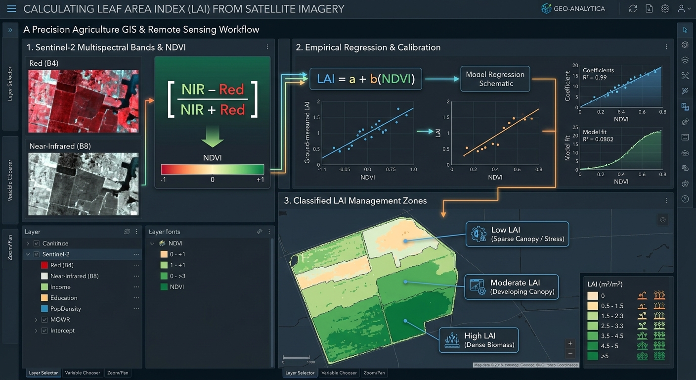
How to Calculate Leaf Area Index (LAI) from Satellite Imagery for Precision Agriculture

 

1. Introduction: Understanding Leaf Area Index in Precision Agriculture

Modern agriculture increasingly relies on satellite remote sensing to monitor crop growth, identify stressed areas, estimate biomass, and improve the efficiency of farm inputs. One important vegetation canopy metric is the Leaf Area Index (LAI), which describes how much leaf area exists relative to the ground area occupied by a crop.

LAI provides useful information about crop canopy development throughout the growing season. When combined with field observations, weather information, and soil data, it can help agricultural specialists identify differences in crop growth and support decisions about irrigation, nutrient management, and yield estimation. Understanding how to **Calculate Leaf Area Index LAI satellite imagery GIS** datasets allows researchers to track canopy development.

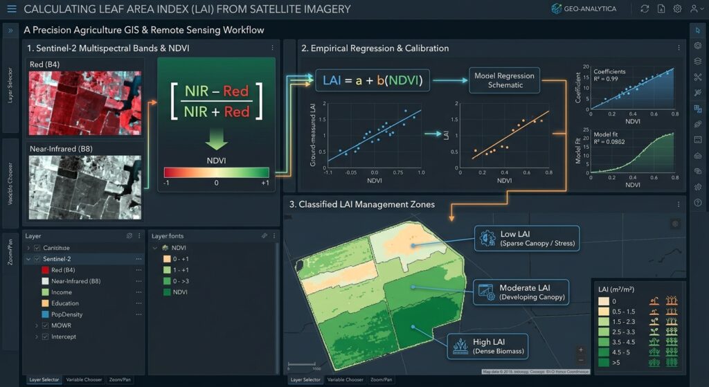
What is Leaf Area Index?

Leaf Area Index (LAI) is the ratio of one-sided green leaf area to the horizontal ground area beneath that vegetation canopy.

[
\boxed{\mathrm{LAI}=\frac{\text{One-sided green leaf area}}{\text{Ground area}}}
]

For example, if a crop canopy has 4 square metres of green leaf area above a 1-square-metre ground plot, its LAI is 4.

LAI is expressed in square metres of leaf area per square metre of ground area (m²/m²). Numerically, it is a dimensionless ratio.

A low LAI may indicate sparse vegetation, early crop development, poor establishment, or stress. A higher LAI generally indicates a denser canopy, although the relationship depends on crop type, growth stage, and environmental conditions.

Why does LAI matter in agriculture?

LAI supports several important agricultural applications:

• Crop health monitoring: Identifying areas with weak canopy development or unusual growth patterns.
• Yield estimation: Providing inputs to crop-growth and statistical yield models.
• Biomass modelling: Helping estimate above-ground biomass when combined with crop-specific relationships and other observations.
• Irrigation management: Tracking canopy development alongside soil moisture, weather, and water-stress indicators.
• Nutrient management: Identifying zones where crop growth differs from expected conditions and where additional investigation may be needed.
• Crop growth monitoring: Comparing canopy development over time to assess the effects of weather, management, and planting conditions.

LAI is not a direct measurement of crop yield or nutrient deficiency. It is a biophysical indicator that becomes more useful when interpreted alongside other data.

This guide explains how to calculate LAI from satellite imagery using QGIS or ArcGIS Pro, focusing on Sentinel-2 data, vegetation indices, empirical regression, and radiative transfer approaches.

2. Methods of Estimating LAI from Satellite Imagery

Satellite sensors measure reflected electromagnetic energy rather than leaf area directly. LAI must therefore be estimated by relating spectral observations to the physical properties of the vegetation canopy. Agronomists often **Calculate Leaf Area Index LAI satellite imagery GIS** pipelines to monitor crop health over large spatial extents.

Two broad approaches are widely used: empirical models and radiative transfer models.

2.1 Empirical regression models

An empirical model establishes a statistical relationship between satellite observations and LAI measurements collected in the field. When building regression models, analysts who **Calculate Leaf Area Index LAI satellite imagery GIS** workflows must ensure high ground-truth correlation.

A common starting point is the Normalized Difference Vegetation Index (NDVI).

[
\boxed{\mathrm{NDVI}=\frac{NIR-Red}{NIR+Red}}
]

Where:

• NIR is near-infrared reflectance.
• Red is red-band reflectance.

Healthy green vegetation usually absorbs much of the red light used in photosynthesis and reflects strongly in the NIR region. NDVI captures this contrast and acts as a useful indicator of vegetation greenness.

However, NDVI is not LAI. To estimate LAI, the index must be converted using a regression model calibrated with field measurements or an appropriate validated reference dataset.

Common empirical model forms

A simple linear model is:

[
\boxed{\mathrm{LAI}=a+b(\mathrm{NDVI})}
]

An exponential model is another option:

[
\boxed{\mathrm{LAI}=a,e^{b(\mathrm{NDVI})}}
]

Here, (a) and (b) are model coefficients fitted to reference data. They are not universal constants and must not be transferred between crops or locations without evaluation.

Advantages: Empirical models are relatively easy to implement in QGIS or ArcGIS Pro and can work well when field measurements and satellite imagery are carefully matched.

Limitations: Model performance depends on the crop, growth stage, soil background, sensor, and quality of the reference measurements. NDVI also tends to saturate in dense vegetation, making it less sensitive to additional increases in LAI at high canopy density.

2.2 Radiative transfer models and Sentinel-2 red-edge bands

A radiative transfer model (RTM) simulates how electromagnetic radiation interacts with leaves, vegetation canopies, and sometimes the atmosphere. The model is then used to infer likely canopy properties from measured satellite reflectance.

One widely used canopy model is PROSAIL, which combines leaf optical properties with canopy radiative transfer.

In practice, a retrieval algorithm compares observed reflectance with model simulations or uses a trained model to estimate LAI. Some approaches use look-up tables, while others use neural networks or other machine-learning algorithms trained using simulated spectra.

Why use Sentinel-2 red-edge bands?

The Sentinel-2 satellite mission includes red-edge bands that help capture changes in vegetation reflectance associated with canopy structure and leaf biochemistry.

Sentinel-2 band	Spectral region	Agricultural relevance	Native resolution
B4	Red	Vegetation absorption; useful for NDVI	10 m
B5	Red edge	Canopy and chlorophyll-related information	20 m
B6	Red edge	Vegetation condition and canopy variation	20 m
B7	Red edge	Additional canopy spectral information	20 m
B8	Near-infrared	Vegetation structure and NDVI	10 m
B8A	Narrow near-infrared	Canopy information at a 20 m grid	20 m

Red-edge information can improve LAI estimation, particularly where conventional vegetation indices become less sensitive to changes in dense crop canopies.

For a practical alternative to developing your own radiative transfer model, ESA’s SNAP Biophysical Processor estimates LAI and other vegetation variables from Sentinel-2 Level-2A data. Its standard processor uses multiple spectral bands at 20 m resolution and is calibrated for top-of-canopy reflectance, with slope-effect-corrected reflectance recommended for optimal results.

Which method should you choose?

Use empirical regression when you have reliable field measurements and need a crop-specific model that can be reproduced in a GIS calculator. Consider an RTM-based or validated biophysical processor when you need a more physically grounded LAI retrieval that uses multiple spectral bands.

3. Data Requirements

Before processing imagery, prepare the satellite data and supporting datasets. Datasets required to **Calculate Leaf Area Index LAI satellite imagery GIS** files include surface reflectance rasters and vector boundaries.

Satellite imagery

For most field-scale precision agriculture projects, Sentinel-2 is a practical starting point because it provides multispectral imagery at 10 m and 20 m resolution.

Download Sentinel-2 Level-2A surface reflectance imagery from the Copernicus Data Space Browser.

Choose an image with low cloud cover during the crop growth stage you want to assess. For seasonal monitoring, obtain multiple acquisitions across the growing season.

You may also use Landsat 8/9 imagery. However, its principal multispectral bands have a 30 m resolution, which may be too coarse for some small-field or within-field applications.

Supporting data

For an empirical LAI model, you should ideally have:

• Field LAI measurements: Collected using suitable ground instruments or a documented field sampling method.
• Crop information: Crop type, planting date, growth stage, and management practices.
• Field boundaries: Polygons defining the agricultural fields.
• Reference records: Soil properties, irrigation observations, or yield information where available.

Field measurements should be collected as close as possible to the satellite acquisition date. Satellite pixels and field plots must also be spatially matched appropriately.

Software

You can complete the GIS workflow with:

• QGIS: Open-source GIS software with a Raster Calculator.
• ArcGIS Pro: Commercial GIS software with raster map algebra tools.
• ESA SNAP: Useful for applying the Sentinel-2 Biophysical Processor to retrieve LAI directly from suitable input imagery.

4. Step-by-Step Workflow: Calculate LAI in QGIS and ArcGIS Pro

The following workflow uses Sentinel-2 imagery to calculate NDVI, convert NDVI to LAI using a calibrated empirical relationship, and classify the resulting LAI raster into agricultural management zones.

Step 1: Import and prepare multispectral imagery

Begin by downloading a suitable Sentinel-2 Level-2A product. Proper preparation of band layers makes it easier to **Calculate Leaf Area Index LAI satellite imagery GIS** layers accurately.

For an NDVI-based LAI model, you need:

• B4: Red reflectance.
• B8: Near-infrared reflectance.

For a red-edge-based retrieval, you may also need B5, B6, B7, and B8A, depending on your chosen model.

In QGIS

1. Open QGIS and create a new project.
2. Select Layer → Add Layer → Add Raster Layer.
3. Load the required Sentinel-2 bands.
4. Rename the layers clearly, such as Red_B4 and NIR_B8.
5. Add your field-boundary polygon if one is available.

In ArcGIS Pro

1. Create a new project and open a map.
2. Select Map → Add Data.
3. Add the required band rasters.
4. Add the agricultural field-boundary layer.

Before proceeding, mask clouds and cloud shadows using the product’s quality information. Check the image for haze, invalid pixels, and other artefacts.

For reflectance products, inspect the data scaling and metadata. Sentinel-2 surface reflectance values are commonly distributed as scaled integers in downloaded products. Confirm whether scaling has already been applied before treating stored numbers as reflectance.

Step 2: Align the raster bands and study area

Raster arithmetic requires compatible inputs. All bands used in the same calculation should have consistent spatial alignment, dimensions, and pixel resolution.

Sentinel-2 B4 and B8 are both native 10 m bands, making them convenient for NDVI.

For models using red-edge bands, remember that B5, B6, and B7 are native 20 m bands. If the retrieval model requires these bands, use the model’s prescribed grid and resampling settings rather than assuming every output is naturally 10 m.

If alignment is necessary, use the relevant GDAL tools through Processing Toolbox → Align Rasters or Warp (Reproject) in QGIS. In ArcGIS Pro, use appropriate raster resampling and environment settings.

Clip the analysis to the field boundary where appropriate, ensuring that the extent and grid are consistent throughout the workflow. Ensuring proper spatial alignment is essential when you **Calculate Leaf Area Index LAI satellite imagery GIS** deliverables across multiple dates.

Step 3: Calculate NDVI as an intermediate proxy

NDVI provides a simple way to summarize vegetation greenness before estimating LAI.

The formula is:

[
\boxed{\mathrm{NDVI}=\frac{B8-B4}{B8+B4}}
]

Here, Sentinel-2 B8 represents NIR reflectance and B4 represents red reflectance.

In QGIS

1. Select Raster → Raster Calculator.
2. Enter the following expression, adjusting the layer names to match your project:

("NIR_B8@1" - "Red_B4@1") /
("NIR_B8@1" + "Red_B4@1")

3. Set the output path to NDVI.tif.
4. Select the appropriate output extent and pixel resolution.
5. Run the calculation.

QGIS creates an NDVI raster in which each valid pixel contains a calculated vegetation-index value. See the QGIS Raster Analysis documentation for details on the Raster Calculator.

In ArcGIS Pro

1. Open Analysis → Tools.
2. Search for Raster Calculator.
3. Enter an equivalent map algebra expression using the names of your red and NIR raster layers:

Float("NIR_B8" - "Red_B4") /
Float("NIR_B8" + "Red_B4")

4. Set the output raster to NDVI.tif.
5. Configure the output coordinate system, cell size, extent, and snap raster where appropriate.
6. Run the tool.

The Float function helps retain decimal precision. ArcGIS Pro provides further details in its Raster Calculator documentation.

Quality check: Inspect the NDVI output for unexpected gaps or extreme values. Pixels with a zero denominator or invalid input data should be treated as NoData rather than as meaningful vegetation measurements. Intermediate vegetation indices generated before you **Calculate Leaf Area Index LAI satellite imagery GIS** values help evaluate baseline greenness.

Step 4: Convert NDVI into LAI using an empirical model

This step transforms the vegetation index into an estimate of leaf area.

The critical requirement is a suitable model. There is no single universal NDVI-to-LAI formula that produces reliable LAI values for every crop and region. The conversion coefficients must be fitted to appropriate measurements or taken from a validated model whose conditions match your project.

Suppose field measurements and matched satellite observations have been used to fit the following linear relationship:

[
\boxed{\mathrm{LAI}=a+b(\mathrm{NDVI})}
]

For a worked example only, assume the calibration exercise produced:

[
\mathrm{LAI}=0.35+5.1(\mathrm{NDVI})
]

These coefficients are illustrative; they are not a recommended universal conversion for agricultural fields.

If a pixel has NDVI of 0.62, the estimated LAI would be:

[
\mathrm{LAI}=0.35+5.1(0.62)
]

[
\mathrm{LAI}=0.35+3.162=3.512
]

The resulting estimate is approximately 3.51 m²/m².

In a real project, replace these example coefficients with coefficients from your own crop-specific calibration or an independently validated model. When you **Calculate Leaf Area Index LAI satellite imagery GIS** values via regression, ensure your coefficients are properly calibrated.

In QGIS

1. Open Raster → Raster Calculator.
2. Enter the calibrated expression:

0.35 + (5.1 * "NDVI@1")

3. Save the output as LAI_Empirical.tif.
4. Run the calculation.

Remember to replace 0.35 and 5.1 with the coefficients of your actual regression model before using the output operationally.

If your validated model uses an exponential relationship, the expression must match that model’s form, coefficients, and expected units.

In ArcGIS Pro

Open Analysis → Tools → Raster Calculator and enter:

0.35 + (5.1 * "NDVI")

Set the output to LAI_Empirical.tif and run the tool.

Again, this is a demonstration of the calculator syntax, not a universally valid LAI retrieval.

Validate the empirical model

Use independent field measurements to assess how well the predicted LAI matches observed LAI.

Common performance measures include the coefficient of determination ((R^2)), root mean square error (RMSE), and mean absolute error (MAE).

[
\mathrm{RMSE}=
\sqrt{\frac{1}{n}\sum_{i=1}^{n}
(\widehat{LAI}_i-LAI_i)^2}
]

Here, (\widehat{LAI}_i) is the model estimate and (LAI_i) is the observed field measurement.

Use a separate validation dataset where possible. A strong fit to training data alone does not demonstrate that the model will generalize to another season, farm, or crop type.

Step 5: Retrieve LAI with a red-edge biophysical processor

For Sentinel-2 imagery, a biophysical retrieval model can be preferable to a simple NDVI conversion, especially for dense crop canopies.

One practical option is the Sentinel-2 Biophysical Processor available in ESA SNAP.

1. Open SNAP and load a suitable Sentinel-2 Level-2A product.
2. Prepare the reflectance inputs according to the processor documentation, including appropriate corrections for slope effects where needed.
3. Open the available Biophysical Processor.
4. Select the correct Sentinel-2 sensor configuration.
5. Enable Compute LAI.
6. Set the target product and output resolution supported by the processor.
7. Run the processing and inspect the resulting LAI band.
8. Export the LAI output to a GIS-compatible format, such as GeoTIFF, for use in QGIS or ArcGIS Pro.

This approach differs from the empirical workflow because LAI is retrieved from a multiband model rather than calculated by multiplying NDVI by a simple coefficient.

Consult the SNAP Biophysical Processor documentation for current input requirements and processor settings.

Even with a physically based retrieval algorithm, validate results against field measurements when possible. Algorithm assumptions, crop structure, acquisition geometry, and canopy conditions can affect the estimates. Advanced users who **Calculate Leaf Area Index LAI satellite imagery GIS** outputs via radiative transfer models can leverage multiband processors.

Step 6: Classify LAI into crop-management zones

A continuous LAI raster shows spatial variation throughout the field. To support precision agriculture, you can classify it into management zones for further investigation.

A simple relative classification might use:

Zone	Relative LAI pattern	Potential interpretation
Low LAI	Lowest values within the field	Sparse canopy, delayed development, stress, or crop establishment problems
Moderate LAI	Intermediate values	Developing or moderately dense crop canopy
High LAI	Highest values within the field	Dense canopy and potentially strong vegetative growth

These classes are relative examples rather than universal agronomic thresholds. Expected LAI depends on crop species, cultivar, growth stage, planting density, and local growing conditions.

In QGIS

1. Right-click LAI_Empirical or your validated LAI raster.
2. Select Properties → Symbology.
3. Choose Singleband pseudocolor.
4. Select a graduated colour ramp.
5. Set breakpoints based on validated crop thresholds or meaningful field-specific quantiles.
6. Label the classes clearly and apply the symbology.

In ArcGIS Pro

1. Select the LAI raster in the Contents pane.
2. Open the Symbology pane.
3. Choose a suitable graduated colour scheme for the continuous values.
4. Set classification method and class breaks based on the crop and management objective.
5. Label the classes and save the map.

For management-zone analysis, calculate zonal statistics or summarize LAI values within field polygons. This helps identify which fields or parts of fields consistently exhibit low or high canopy development.

Do not interpret a low-LAI zone as a nutrient-deficient zone without corroborating evidence. Low values may also result from drought, pests, disease, compaction, uneven emergence, waterlogging, or image contamination.

5. Real-World Applications in Precision Agriculture

LAI becomes particularly valuable when its spatial and temporal patterns are combined with information about soil, crop stage, and farm management.  Precision farming decisions that rely on data to **Calculate Leaf Area Index LAI satellite imagery GIS** metrics improve input efficiency significantly.

5.1 Variable-rate fertilizer application

Variable-rate fertilizer application aims to match nutrient inputs to differences in crop requirements within a field.

An LAI map can help identify areas with unusually low canopy development, which may indicate a need for further investigation. Agricultural specialists can then compare the map with soil tests, nutrient observations, crop-stage information, yield records, and field scouting.

For example, an area with persistently low LAI despite adequate soil moisture may warrant checking for nutrient deficiencies, poor establishment, or root constraints.

However, LAI alone should not determine fertilizer rates. A low-LAI patch could be caused by drought or waterlogging rather than a lack of nutrients. Use the map as a diagnostic layer within a broader agronomic decision process.

5.2 Drought stress detection

LAI can help track changes in crop canopy development during dry periods. A decrease or slower-than-expected increase in LAI may indicate that crop growth is being affected by water limitations.

A useful monitoring workflow involves:

1. Calculating LAI for several dates throughout the growing season.
2. Comparing each image with the expected growth pattern for the crop.
3. Identifying zones with declining or persistently low LAI.
4. Cross-referencing these zones with rainfall, soil-moisture measurements, irrigation records, and weather observations.
5. Investigating suspected stress areas in the field.

Because LAI changes can lag behind the onset of water stress, supplement it with other indicators such as canopy temperature, soil moisture, and water-related vegetation indices.

5.3 Crop growth and yield estimation

LAI is useful for monitoring crop development and can be incorporated into crop-growth models that simulate light interception, biomass accumulation, and yield.

Repeated observations are particularly valuable because a single image may not capture the crop’s development trajectory. A time series helps distinguish temporary spatial differences from persistent growth limitations.

Yield estimation still requires an appropriate crop-specific model and, ideally, historical yield or field-observation data. LAI should be treated as an input or indicator rather than a direct replacement for harvest measurements.

6. Common Errors and Quality Checks

Using an uncalibrated NDVI-to-LAI equation: A formula published for another crop or region may perform poorly. Fit and validate the regression with suitable reference data.

Ignoring reflectance scaling: Incorrectly interpreting stored digital numbers can produce invalid indices and model outputs. Check the satellite product metadata before processing.

Mixing spatial resolutions without planning: Red-edge bands often have a coarser native resolution than red and NIR bands. Follow the chosen model’s required grid and do not imply that resampling creates additional spatial information.

Ignoring clouds and shadows: These features distort reflectance and can be mistaken for crop stress. Apply quality masks and inspect the image before generating LAI.

Assuming higher LAI always means healthier crops: Very dense canopies, lodging, crop maturity, and other conditions can complicate interpretation. Consider the crop’s growth stage and management objective.

Treating every low-LAI zone as a fertilizer problem: Confirm suspected causes using agronomic observations and other spatial data before changing input rates.

7. Summary and Takeaways

Calculating Leaf Area Index from satellite imagery provides a practical way to assess crop canopy development across agricultural fields.

The workflow begins with suitable multispectral imagery, followed by reflectance preparation, vegetation-index calculation, and conversion to LAI through a calibrated empirical model or a biophysical retrieval algorithm. The resulting raster can be classified into relative crop-management zones and monitored over time.

For precision agriculture, the most important distinction is between a vegetation index and a biophysical estimate. NDVI can act as a useful proxy, but it does not measure LAI directly. Reliable LAI maps require an appropriate retrieval method, consistent satellite processing, and validation against suitable reference data.

When combined with field scouting, soil measurements, weather information, and crop-growth knowledge, LAI can support better-informed decisions about nutrient management, irrigation, and crop monitoring.

Further Resources

• ESA SNAP Biophysical Processor — Sentinel-2 LAI and other vegetation-variable retrievals.
• Copernicus Data Space Browser — Access Sentinel-2 imagery.
• QGIS Raster Analysis Documentation — Raster Calculator and raster-processing guidance.
• ArcGIS Pro Raster Calculator — Raster map algebra for LAI workflows.
• PROSAIL-based LAI retrieval research — Research on physical and hybrid approaches to estimating LAI from Sentinel-2 observations.