Table of Contents

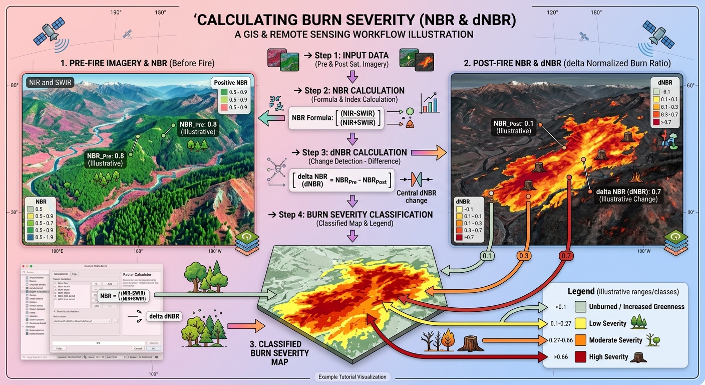
Calculating Burn Severity with Normalized Burn Ratio (NBR) in QGIS: A Step-by-Step Tutorial

1. Introduction: Understanding Burn Severity with Satellite Remote Sensing

To successfully Calculate Burn Severity NBR QGIS workflows, environmental scientists must understand how wildfires transform vegetation and soil. Wildfires can transform vegetation, expose bare soil, alter soil moisture, and affect ecosystem recovery. Understanding the spatial distribution of these changes is essential for environmental monitoring, forest management, watershed protection, and post-fire rehabilitation.

Satellite remote sensing provides an efficient way to assess wildfire impacts across large areas. Instead of relying exclusively on field surveys, researchers can compare satellite imagery acquired before and after a fire to identify changes in vegetation and surface conditions.

One of the most widely used methods is the Normalized Burn Ratio (NBR), a spectral index that highlights differences between near-infrared and shortwave infrared reflectance.Learning how to **Calculate Burn Severity NBR QGIS** allows researchers to assess wildfire impacts efficiently.

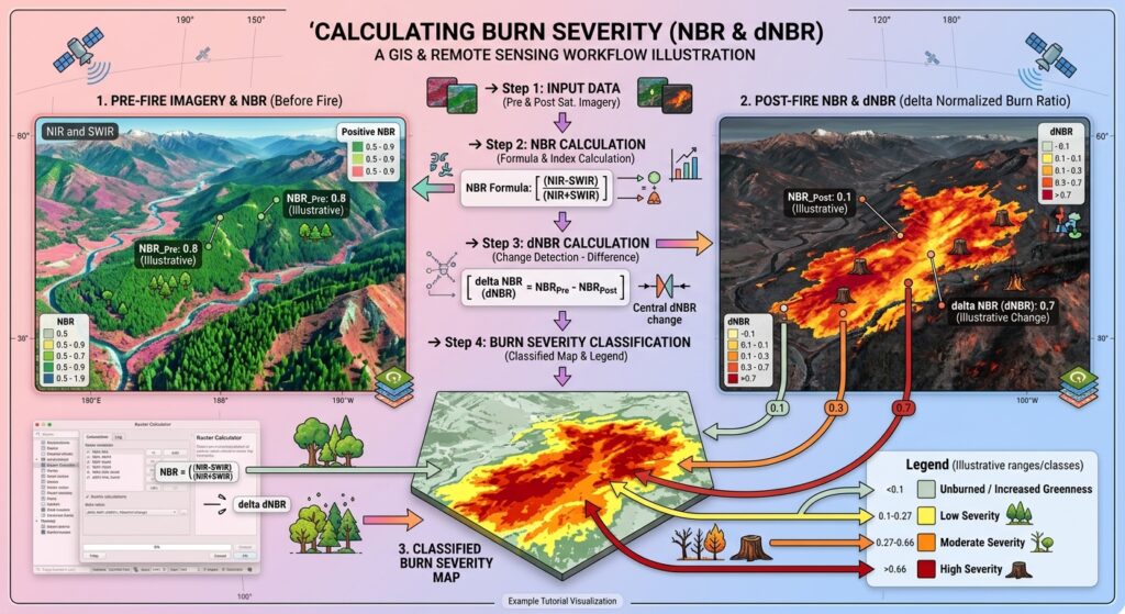
What is burn severity?

Burn severity describes the degree to which a fire alters vegetation, organic matter, and soil conditions. It is different from fire intensity, which relates to the energy released during combustion.

Low-severity burning may scorch vegetation while leaving much of the overstory intact. High-severity burning may consume vegetation and litter extensively, expose mineral soil, and cause substantial tree mortality.

Satellite-derived burn severity estimates indicate changes in surface conditions associated with fire. They do not directly measure every ecological effect, such as soil heating or below-ground root mortality.

Why are NIR and SWIR important?

NBR uses two parts of the electromagnetic spectrum:

Near-infrared (NIR): Healthy vegetation typically reflects strongly in the NIR region because of its internal leaf structure.
Shortwave infrared (SWIR): Reflectance is influenced by vegetation water content, exposed soil, and burned surface materials. Healthy vegetation generally absorbs more SWIR energy than dry or damaged vegetation.

After a wildfire, vegetation damage and changes in surface moisture often reduce NIR reflectance and increase SWIR reflectance. Consequently, NBR commonly decreases in burned areas.

The U.S. Geological Survey (USGS) identifies NBR as an important index for burned-area identification and burn-severity assessment.

This tutorial demonstrates how to calculate pre-fire and post-fire NBR, derive Delta NBR (dNBR), classify burn severity, and validate the resulting map using QGIS.

2. Data Requirements

Before starting, prepare the satellite imagery and GIS layers required for your study.

2.1 Satellite imagery

You can use either Sentinel-2 or Landsat 8/9 imagery. For a beginner-friendly project, choose atmospherically corrected surface reflectance products rather than uncorrected digital imagery.

Satellite	NIR band	SWIR2 band	Native pixel size
Sentinel-2 MSI	B8A, or B8 with appropriate resampling	B12	B8A: 20 m; B8: 10 m; B12: 20 m
Landsat 8/9 OLI	Band 5	Band 7	30 m for both bands

For Sentinel-2, using B8A and B12 is convenient because both bands have a native 20 m resolution. If you use B8 instead, align it to the 20 m SWIR2 grid for a 20 m NBR output.

For Landsat 8/9, use Band 5 for NIR and Band 7 for SWIR2.

2.2 Where to download the imagery

Use one of these official sources:

Copernicus Data Space Browser for Sentinel-2 Level-2A imagery.
USGS EarthExplorer for Landsat Collection 2 Level-2 surface reflectance products.

Download two suitable images: one acquired before the fire and another acquired after it.

Choose images with minimal cloud cover, similar seasonal conditions, and acquisition dates appropriate to the fire and ecological response you are investigating.

For Sentinel-2, use the Scene Classification Layer (SCL) to identify clouds, cloud shadows, and other unsuitable pixels. For Landsat, use the QA_PIXEL quality band to mask clouds, shadows, snow, and fill pixels.

Important: Reflectance scaling matters. Landsat Collection 2 Level-2 surface reflectance uses the conversion:

[
\rho = DN \times 0.0000275 – 0.2
]

where (\rho) is surface reflectance and (DN) is the stored pixel value. Apply this scaling before calculating NBR. For Sentinel-2, check the product metadata for the applicable reflectance scale and any band-specific additive offsets. Do not assume raw digital numbers are always physical reflectance.

Refer to the USGS Landsat scaling guidance and Copernicus Sentinel-2 documentation.

2.3 GIS software and supporting layers

You will need:

QGIS installed on your computer.
The pre-fire and post-fire NIR and SWIR2 raster bands.
A fire-perimeter polygon, if available.
Optional reference data, such as field observations, high-resolution imagery, or official burned-area products.

Ensure that the relevant rasters use a consistent coordinate reference system, spatial extent, pixel size, and grid alignment.

3. Step-by-Step Workflow: Calculate Burn Severity NBR in QGIS

Step 1: Download and prepare cloud-free imagery

Open the Copernicus Data Space Browser or USGS EarthExplorer and identify the fire location.

For Sentinel-2:

Select a pre-fire acquisition and a post-fire acquisition.
Prefer Level-2A surface reflectance products.
Download the relevant NIR and SWIR2 bands: B8A and B12 for a straightforward 20 m workflow.
Use the SCL layer to identify and mask cloud, cloud-shadow, snow, and invalid pixels.

For Landsat 8/9:

Select pre-fire and post-fire Collection 2 Level-2 scenes.
Download surface reflectance Band 5 and Band 7.
Apply the documented reflectance scale and offset.
Use QA_PIXEL to mask clouds, shadows, snow, and fill pixels.

Extract the downloaded archives and load the bands into QGIS.

QGIS navigation: Layer → Add Layer → Add Raster Layer

Browse to your downloaded raster files and add them to the map. Rename them clearly, for example:

Pre_NIR
Pre_SWIR2
Post_NIR
Post_SWIR2

If the pre-fire and post-fire rasters are not aligned, use Raster → Projections → Warp (Reproject) or the relevant GDAL alignment tools to establish a common CRS, extent, pixel size, and grid. For Sentinel-2 B8/B12 combinations, avoid treating a resampled 10 m output as though the 20 m SWIR band provides true 10 m spatial detail.

Step 2: Calculate the Normalized Burn Ratio (NBR)

NBR is calculated separately for each date using NIR and SWIR2 surface reflectance.

Mathematical formula:

[
\boxed{\mathrm{NBR}=\frac{\mathrm{NIR}-\mathrm{SWIR2}}{\mathrm{NIR}+\mathrm{SWIR2}}}
]

Calculate the index for both dates:

[
\mathrm{NBR}{pre}=
\frac{\mathrm{NIR}{pre}-\mathrm{SWIR2}{pre}}
{\mathrm{NIR}{pre}+\mathrm{SWIR2}_{pre}}
]

[
\mathrm{NBR}{post}=
\frac{\mathrm{NIR}{post}-\mathrm{SWIR2}{post}}
{\mathrm{NIR}{post}+\mathrm{SWIR2}_{post}}
]

NBR generally ranges between −1 and +1 when calculated from suitable reflectance values. Higher positive values often correspond to healthy vegetation, whereas lower values may indicate burned surfaces, sparse vegetation, water, or other non-vegetated conditions.

Calculate pre-fire NBR

Open Raster → Raster Calculator.
In the raster bands list, select the pre-fire NIR and SWIR2 layers.
Enter the expression below, replacing the example layer names with the names shown in your QGIS project.

("Pre_NIR@1" - "Pre_SWIR2@1") /
("Pre_NIR@1" + "Pre_SWIR2@1")

Set the output file to NBR_Pre.tif.
Confirm the output extent and resolution are appropriate for the input grid.
Click OK or Run, depending on the QGIS calculator you are using.

QGIS calculates the expression for each valid pixel and saves the resulting raster. See the QGIS Raster Calculator documentation.

Calculate post-fire NBR

Repeat the same workflow using the post-fire bands:

("Post_NIR@1" - "Post_SWIR2@1") /
("Post_NIR@1" + "Post_SWIR2@1")

Save the output as NBR_Post.tif.

You should now have two NBR layers showing vegetation and surface conditions before and after the fire.

Quality check: Inspect both rasters using a suitable colour ramp. Investigate unexpected extreme values, NoData gaps, or stripes before continuing. The denominator should not be zero, and cloud or shadow contamination can produce misleading results. When you **Calculate Burn Severity NBR QGIS** using the raster calculator, ensure your band math syntax is correct.

Step 3: Calculate Delta NBR (dNBR)

A single NBR image describes surface conditions on one date. To investigate changes associated with a fire, calculate the difference between the two images.

Delta NBR (dNBR) is defined as:

[
\boxed{\mathrm{dNBR}=\mathrm{NBR}{pre}-\mathrm{NBR}{post}}
]

This order is important: subtract the post-fire NBR from the pre-fire NBR.

A large positive dNBR often indicates a substantial decline in NBR following the fire, which may be associated with greater burn severity. Values near zero suggest relatively little change, while negative values indicate that NBR increased after the event. That increase may reflect vegetation recovery, seasonal differences, or other changes rather than an absence of fire.

Calculate dNBR in QGIS

Open Raster → Raster Calculator.
Select the pre-fire and post-fire NBR layers.
Enter:

"NBR_Pre@1" - "NBR_Post@1"

Save the output as dNBR.tif.
Run the calculation.

The resulting raster contains continuous dNBR values rather than named burn-severity categories.

For example, if a pixel has pre-fire NBR of 0.72 and post-fire NBR of 0.18:

[
\mathrm{dNBR}=0.72-0.18=0.54
]

This indicates a marked decline in NBR, but the appropriate severity class must be interpreted using suitable thresholds and, ideally, local validation.

Important: dNBR may also be stored in a scaled form, such as dNBR multiplied by 1,000. The threshold values must match the scale of your raster. The classification thresholds below apply to unscaled dNBR values.

Step 4: Classify burn severity

Continuous dNBR is useful for analysis, but a classified map makes the results easier to interpret and communicate.

Burn-severity thresholds vary with ecosystem type, pre-fire vegetation, image timing, sensor, and assessment methods. The following is a simplified four-class starting point based on commonly cited dNBR intervals; it is not a universal classification for every wildfire.

dNBR value	Simplified class	General interpretation
Less than 0.10	Unburned / no positive severity signal	No clear positive burn-change signal; negative values may indicate increased greenness
0.10 to less than 0.27	Low severity	Relatively small NBR decline
0.27 to less than 0.66	Moderate severity	Intermediate NBR decline; combines moderate-low and moderate-high classes
0.66 or greater	High severity	Large NBR decline, potentially indicating severe vegetation or surface change

These simplified boundaries merge the two moderate classes used in some established schemes. The USGS and Monitoring Trends in Burn Severity (MTBS) guidance emphasizes that burn-severity classes and thresholds may be tailored to the fire, ecological conditions, and available field data. Validating outputs when you **Calculate Burn Severity NBR QGIS** ensures your severity classes match field observations.

Option A: Classify the dNBR raster using symbology

This is the simplest option when you want a visual map without creating a separate integer raster.

Right-click dNBR and choose Properties.
Select Symbology.
Choose Singleband pseudocolor.
Set the interpolation and classification mode appropriately, using discrete ranges where supported.
Create class breaks at −0.10 if you are separately displaying increased greenness, then 0.10, 0.27, and 0.66 for the simplified positive-severity classes.
Apply meaningful labels and colours.

A negative-to-low dNBR area should not automatically be labelled “unburned” if evidence suggests regrowth or a seasonal change. If those distinctions matter to your research, add a separate increased-greenness class.

Option B: Create a four-class raster using Raster Calculator

To create a numerical raster with class codes, open Raster → Raster Calculator and enter:

if("dNBR@1" < 0.10, 1,
   if("dNBR@1" < 0.27, 2,
      if("dNBR@1" < 0.66, 3, 4)))

Save the output as Burn_Severity_4class.tif.

The codes represent:

1 = Unburned / no positive severity signal
2 = Low severity
3 = Moderate severity
4 = High severity

This expression assumes that dNBR is in unscaled decimal form and that invalid pixels are properly represented as NoData. Review how your selected Raster Calculator handles NoData, and mask invalid pixels before classification if necessary.

To style the result, open Layer Properties → Symbology, choose Paletted/Unique values where available, and assign a distinct label and colour to each code. A conventional scheme uses a muted neutral colour for class 1, yellow for low severity, orange for moderate severity, and dark red for high severity.

4. Validating Your Burn-Severity Map

A classified dNBR raster is an estimate derived from spectral change. Before using it in an environmental report, check whether the mapped patterns make sense.

4.1 Cross-reference the fire perimeter

Load an official fire-perimeter polygon into QGIS:

Layer → Add Layer → Add Vector Layer

Overlay the perimeter on your dNBR and burn-severity maps. Check whether high-change zones broadly correspond to the known burned area and whether unexpected patterns occur outside the perimeter.

A perimeter is a useful reference, but it is not definitive proof of burn severity. It may contain unburned islands or differ spatially from the area where fire effects are visible in satellite imagery.

4.2 Compare pre-fire and post-fire imagery

Use the RGB or false-colour imagery for both dates to inspect the vegetation changes underlying the dNBR result. Investigate isolated high-severity patches, abrupt class boundaries, and areas affected by clouds or shadows.

4.3 Use ground observations where possible

Field observations, geotagged photographs, vegetation surveys, and evidence of soil or canopy damage can help assess the map.

For formal studies, consider field-based burn-severity measures such as the Composite Burn Index (CBI) and evaluate how well the classified map agrees with observations. If sufficient reference data are available, calculate a confusion matrix and class-specific accuracy statistics.

4.4 Document your method

Record the satellite and product level, acquisition dates, bands, scaling and masking procedures, output resolution, dNBR formula, class thresholds, and validation data. This information is essential for reproducible environmental research.

5. Common Errors to Avoid

Using mismatched dates: Seasonal vegetation changes may be misinterpreted as fire effects. Select appropriate pre-fire and post-fire scenes and document the timing.

Ignoring clouds and shadows: These can cause incorrect NBR values. Apply quality masks before calculating the index.

Using raw Landsat Collection 2 values: Their multiplicative scaling factor and additive offset must be applied before NBR calculation.

Mixing band resolutions: Align the NIR and SWIR2 bands to a common grid without claiming greater spatial detail than the coarser input supports.

Treating thresholds as universal: Thresholds developed for one ecosystem or study may not transfer directly to another. Validate or calibrate them for the study area.

Confusing spectral change with ecological severity: dNBR captures changes in spectral response, not every ecological process caused by a fire.

Avoiding common preprocessing mistakes ensures you successfully **Calculate Burn Severity NBR QGIS** every time.

6. Summary and Takeaways

Calculating burn severity in QGIS provides a practical entry point into remote sensing-based wildfire assessment.

The workflow is straightforward: acquire cloud-masked pre-fire and post-fire surface reflectance, calculate NBR from NIR and SWIR2, subtract post-fire NBR from pre-fire NBR to create dNBR, and classify the result using defensible thresholds.

For environmental research projects, the most important lesson is that accurate burn-severity mapping depends on more than the index formula. Consistent imagery, correct reflectance scaling, cloud masking, aligned rasters, appropriate thresholds, and validation are all necessary for defensible results.

The resulting dNBR and classified severity rasters can support post-fire vegetation assessment, erosion-risk investigations, ecosystem recovery monitoring, and environmental management when interpreted alongside other evidence.