Moran’s I Spatial Autocorrelation: Beginner GIS Guide

If you are working with geographic data, simply knowing where high and low values occur is often not enough. You may also need to determine whether those values are clustered, dispersed, or randomly distributed across space.

This is where Moran’s I spatial autocorrelation becomes useful. Moran’s I provides a statistical way to determine whether nearby geographic features have similar or dissimilar attribute values.

For GIS students, the difficult part is often interpreting the resulting Moran’s I value, z-score, and p-value. This guide breaks the process down step by step and shows how to perform spatial autocorrelation analysis in ArcGIS Pro and QGIS. Whether you are tackling a graded lab or building a spatial model, mastering Moran’s I spatial autocorrelation is an essential milestone for any GIS student or analyst.

What You Will Learn

• What spatial autocorrelation means
• How Moran’s I relates to the First Law of Geography
• Positive, negative, and zero spatial autocorrelation
• Global Moran’s I vs Local Moran’s I
• How spatial weights determine which features are neighbors
• How to run Moran’s I in ArcGIS Pro
• How to perform the analysis in QGIS using PySAL
• How to interpret z-scores and p-values
• How to write the results in a GIS lab report

 

---

What Is Moran’s I Spatial Autocorrelation?

Moran’s I is a statistical measure used to determine whether similar or dissimilar attribute values are spatially clustered. Properly calculating Moran’s I spatial autocorrelation ensures you don’t mistake random noise for genuine geographical patterns.

Imagine a map showing unemployment rates for different counties. If counties with high unemployment tend to be next to other counties with high unemployment, the dataset exhibits positive spatial autocorrelation.

If high values tend to be surrounded by low values and vice versa, the pattern demonstrates negative spatial autocorrelation.

If the values show no meaningful spatial pattern, the result may indicate spatial randomness.

Moran’s I therefore helps answer a fundamental spatial question:

Are nearby locations more similar or different than we would expect by chance?

Moran’s I and the First Law of Geography

Moran’s I is closely related to the famous First Law of Geography, commonly attributed to Waldo Tobler:

Things that are closer together tend to be more related than things that are farther apart.

This principle is fundamental to spatial analysis. When researchers operationalize this geographic principle into quantitative metrics, Moran’s I spatial autocorrelation serves as the industry standard tool.

For example, neighboring communities may experience similar rainfall, soil conditions, land prices, disease rates, or socioeconomic conditions because they share environmental or geographic characteristics.

Moran’s I converts this geographical concept into a statistical measurement.

---

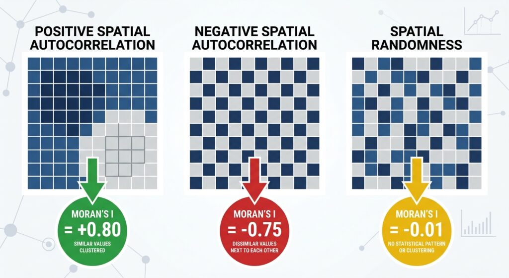
Understanding Positive, Negative, and Zero Spatial Autocorrelation

The easiest way to understand Moran’s I is to think about similarity between neighboring features.

Positive Spatial Autocorrelation

Positive spatial autocorrelation occurs when similar values tend to occur near one another.

Examples include:

• High-income areas next to high-income areas
• High rainfall locations near other high rainfall locations
• High disease rates clustering geographically
• Low property values occurring in neighboring areas

On a map, this often appears as clusters. Detecting these distinct clusters is the primary objective when running Moran’s I spatial autocorrelation on socioeconomic or environmental datasets.

A positive Moran’s I value generally indicates positive spatial autocorrelation.

Negative Spatial Autocorrelation

Negative spatial autocorrelation occurs when neighboring features tend to have dissimilar values.

For example, high-value locations may be surrounded by low-value locations.

This produces a more dispersed or checkerboard-like pattern.

A negative Moran’s I value can indicate negative spatial autocorrelation.

Spatial Randomness

A Moran’s I value close to the expected value under spatial randomness suggests that there may be no statistically significant spatial autocorrelation.

However, don’t interpret a value close to zero automatically as proof of randomness.

You need to examine the statistical significance, particularly the z-score and p-value.

---

Global Moran’s I vs Local Moran’s I

One of the most important concepts for GIS assignments is understanding the difference between Global Moran’s I and Local Moran’s I.

What Is Global Moran’s I?

Global Moran’s I provides a single statistic for the entire study area.

It answers:

Is there an overall spatial pattern in this dataset?

Evaluating this global tendency is why Moran’s I spatial autocorrelation is usually the very first diagnostic GIS analysts perform. For example, you might calculate Global Moran’s I for population density across all counties in a country.

The output might tell you that population density is significantly clustered.

However, Global Moran’s I does not necessarily tell you where the clusters are.

What Is Local Moran’s I?

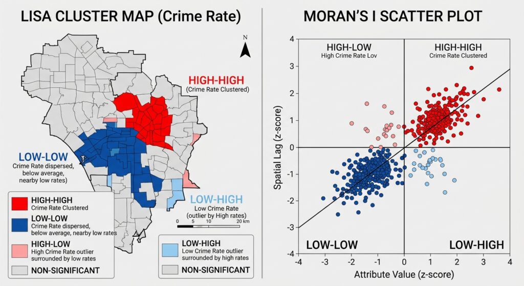
Local Moran’s I examines individual features and identifies localized spatial patterns.

It is commonly associated with Local Indicators of Spatial Association (LISA).

Local Moran’s I can identify patterns such as:

• High-High (HH): a high value surrounded by high values
• Low-Low (LL): a low value surrounded by low values
• High-Low (HL): a high value surrounded by low values
• Low-High (LH): a low value surrounded by high values

The first two are examples of spatial clustering, while High-Low and Low-High locations can identify spatial outliers.

Global vs Local Moran’s I

Characteristic	Global Moran’s I	Local Moran’s I
Analysis scale	Entire study area	Individual features
Main question	Is there overall spatial autocorrelation?	Where are clusters/outliers?
Output	One overall statistic	Statistic for each feature
Useful for	Testing overall pattern	Mapping local clusters
Common interpretation	Clustered/dispersed/random	HH, LL, HL, LH

---

Struggling to set up your spatial weights matrix or interpret your software’s output? You can explore our expert GIS assignment assistance services to get personalized guidance on your spatial statistics workflow.

Understanding Spatial Weights

Before calculating Moran’s I, GIS software needs to know which features should be considered neighbors.

This relationship is represented through a spatial weights matrix.

Think of it as a set of rules answering:

“Which geographic features influence or interact with this feature?”

Two common approaches are contiguity and distance-based relationships. Before diving into the mathematics of Moran’s I spatial autocorrelation, you must define how geographic features interact with one another.

Contiguity-Based Weights

Contiguity defines neighbors according to shared boundaries.

For polygon data, common approaches include:

Rook contiguity: features must share an edge.

Queen contiguity: features can share an edge or a corner.

Choosing the correct contiguity matrix directly dictates how sensitive your final Moran’s I spatial autocorrelation score will be to boundary adjustments. For example, if you are analyzing counties, two counties sharing a boundary may be considered neighbors.

Distance-Based Weights

Distance-based methods define neighbors using geographic distance.

A fixed distance band might specify that features within 50 kilometers are neighbors.

An inverse distance approach gives closer features greater influence than distant features.

This is particularly useful for point data or situations where physical distance is more meaningful than shared boundaries.

Pro Tip: Your spatial weights conceptualization should reflect the geography of your research question. Don’t select Queen contiguity simply because it is the default option if distance is actually more meaningful for your dataset.

---

How to Calculate Moran’s I Spatial Autocorrelation in ArcGIS Pro & QGIS

The workflow is broadly similar in both platforms:

Prepare data → define neighbors → calculate Moran’s I → interpret statistics → map results

Let’s examine each workflow.

---

Running Global Moran’s I in ArcGIS Pro

ArcGIS Pro provides Moran’s I through its Spatial Statistics tools.

Step 1: Prepare Your Dataset

Start with a feature layer containing the variable you want to analyze.

For example:

• population density
• crime rate
• rainfall
• disease incidence
• house prices

Open the attribute table and verify that the analysis field is numeric.

Remove or investigate obvious errors before beginning the analysis.

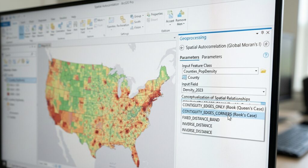
Step 2: Open Spatial Autocorrelation

To begin calculating Moran’s I spatial autocorrelation within ArcGIS Pro, navigate to your Analysis tab.

Open:

Analysis → Tools

Search for:

Spatial Autocorrelation (Global Moran’s I)

This tool calculates Global Moran’s I and provides statistical information about the spatial pattern.

Step 3: Select the Input Features

Choose your polygon or point layer.

Then select the numerical field you want to analyze.

For example:

Population_Density

Step 4: Choose the Conceptualization of Spatial Relationships

This is one of the most important settings.

Depending on your dataset and research question, you may choose a method based on:

• Fixed distance
• Inverse distance
• Contiguity
• Other supported spatial relationship conceptualizations

For polygon administrative areas, contiguity can be appropriate.

For point observations, distance-based relationships may be more suitable.

Step 5: Set the Distance Threshold if Required

If using a fixed-distance method, specify the distance threshold.

The threshold should be large enough that features have meaningful neighbors.

A major problem occurs when some features have zero neighbors.

Pro Tip: Always inspect the resulting messages and parameters. A poor spatial weights configuration can make your statistical interpretation unreliable.

Step 6: Run the Tool

Click Run.

ArcGIS Pro will produce statistics including:

• Moran’s I index
• Expected Moran’s I
• Variance
• z-score
• p-value

---

How to Interpret Moran’s I Results

Structuring a clear write-up for your Moran’s I spatial autocorrelation results requires linking your numerical output directly back to your initial research hypothesis.

Suppose your output produces something similar to:

Statistic	Example
Moran’s I	0.42
Expected I	-0.03
z-score	4.85
p-value	< 0.001

What does this mean?

Step 1: Examine Moran’s I

The positive Moran’s I value suggests positive spatial autocorrelation.

In other words, similar values tend to occur near one another.

Step 2: Examine the z-Score

The z-score tells you how far your observed statistic is from what would be expected under the null hypothesis.

A large positive z-score provides evidence against spatial randomness in favor of positive spatial autocorrelation.

A large negative z-score can indicate significant negative spatial autocorrelation.

Step 3: Examine the p-Value

The p-value helps determine whether the observed pattern is statistically significant.

For example, if:

p < 0.05

you would commonly reject the null hypothesis at the 5% significance level.

But remember:

A significant p-value does not tell you whether the pattern is positive or negative.

You need the Moran’s I value and z-score to understand the direction.

Pro Tip: Never write in your lab report that “p = 0.001 means there is clustering.” The p-value tells you about statistical significance. The direction and nature of the pattern must be interpreted using the Moran’s I statistic and z-score.

---

Running Moran’s I in QGIS Using PySAL

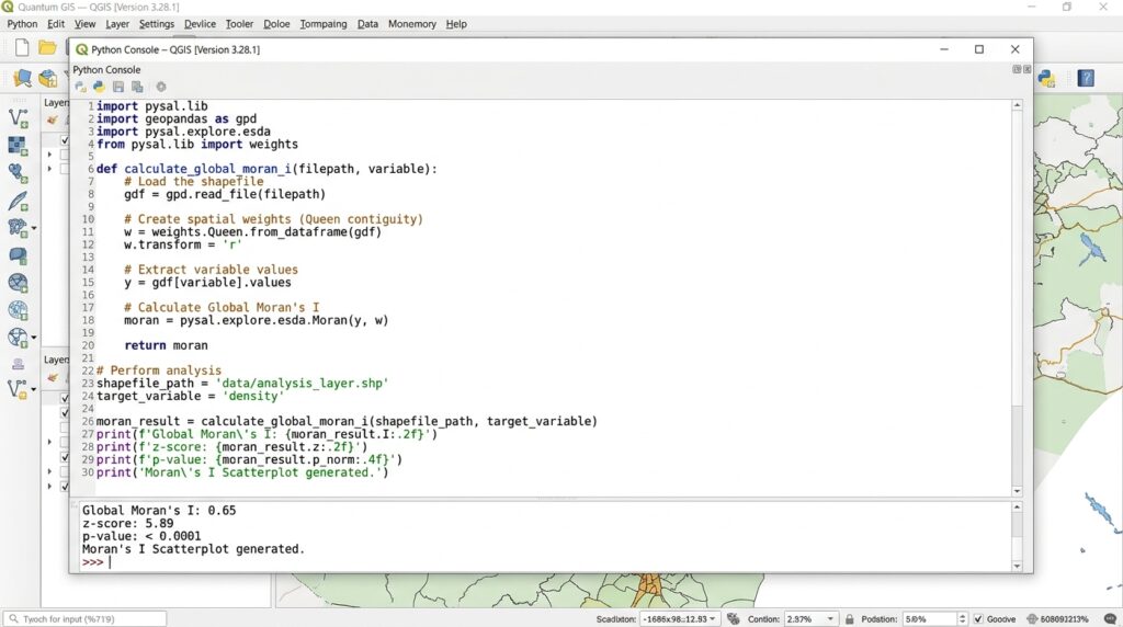
QGIS can be used with Python-based spatial statistics libraries such as PySAL, particularly its esda package for exploratory spatial data analysis.

PySAL is an open-source Python ecosystem designed for spatial analysis.

Step 1: Prepare Your Data

Load your polygon or point layer into QGIS.

Make sure the attribute you want to analyze is numeric.

For example:

crime_rate

or:

rainfall_mm

Step 2: Create a Spatial Weights Structure

In PySAL, spatial weights can be created using different approaches.

For polygon data, you can create contiguity weights such as Queen or Rook.

Conceptually:

from libpysal.weights import Queen

w = Queen.from_dataframe(gdf)

For distance-based point data, you can use distance-based weights.

The appropriate method depends on your dataset and research question.

Step 3: Calculate Global Moran’s I

The esda package provides Moran’s I functionality.

A simplified workflow looks like:

from esda.moran import Moran

mi = Moran(gdf["value"], w)

print(mi.I)
print(mi.z_sim)
print(mi.p_sim)

The exact implementation may depend on your PySAL and GeoPandas versions.

Step 4: Interpret the Output

You can examine:

• I — Moran’s I statistic
• z_sim — simulated z-score
• p_sim — simulated p-value

Interpret these together rather than relying on one statistic.

---

Local Moran’s I and LISA Cluster Analysis

Global Moran’s I tells you whether a spatial pattern exists across the entire study area.

But suppose your professor asks:

“Where are the statistically significant clusters?”

That’s where Local Moran’s I becomes useful.

Step 1: Calculate Local Moran’s I

Using PySAL, the Moran_Local function can calculate local statistics.

A simplified example is:

from esda.moran import Moran_Local

local_moran = Moran_Local(gdf["value"], w)

You can then use the resulting statistics to classify individual observations.

Step 2: Identify Cluster Types

The results can be interpreted using the familiar LISA categories:

Pattern	Meaning
High-High	High value surrounded by high values
Low-Low	Low value surrounded by low values
High-Low	High-value spatial outlier
Low-High	Low-value spatial outlier

Step 3: Map Significant Clusters

Map only statistically significant results when producing a LISA cluster map.

This prevents you from visually presenting every possible local pattern as statistically meaningful.

---

How to Write Moran’s I Results in a GIS Lab Report

A common mistake is reporting only the numerical result.

Instead, connect the statistic to the spatial interpretation.

For example:

“Global Moran’s I produced a positive statistic of 0.42 with a z-score of 4.85 and p < 0.001. The statistically significant positive result indicates that similar population-density values are spatially clustered rather than randomly distributed.”

Notice that the statement includes:

1. Moran’s I
2. z-score
3. p-value
4. Direction of spatial association
5. Plain-language interpretation

This is much stronger than simply writing:

“The Moran’s I value was 0.42.”

---

Common Mistakes When Using Moran’s I

Mistake 1: Ignoring Spatial Weights

Moran’s I depends on how neighboring relationships are defined.

Changing from Queen contiguity to a fixed-distance relationship can change your results.

Always document the spatial weights method. An improper neighborhood definition will quietly invalidate your entire Moran’s I spatial autocorrelation workflow.

Mistake 2: Confusing Statistical Significance With Clustering

A small p-value indicates evidence against the null hypothesis.

It does not independently tell you whether the pattern is clustered or dispersed.

Use the Moran’s I statistic and z-score to determine the direction.

Mistake 3: Using the Wrong Distance Threshold

If your threshold is too small, some features may have no neighbors.

If it is too large, almost every feature may become connected.

The threshold should reflect the geography and scale of your study.

Mistake 4: Forgetting the Unit of Analysis

Moran’s I results depend on the spatial units used.

For example, analyzing population density by counties can produce different results from analyzing it by smaller administrative areas.

This issue is related to the broader modifiable areal unit problem (MAUP).

---

Pro Tips for Interpreting z-Scores and p-Values

Pro Tip 1: Don’t interpret the p-value alone.

Always report Moran’s I, z-score, and p-value together.

Pro Tip 2: State your significance level.

If you use α = 0.05, explain that your conclusion is based on the 5% significance threshold.

Pro Tip 3: Distinguish direction from significance.

A positive z-score doesn’t automatically mean the result is significant. A z-score must be sufficiently far from zero to provide evidence against the null hypothesis.

Pro Tip 4: Explain the geography.

Statistical significance is more meaningful when you can connect it to the actual geography of your study.

---

External Resources for Further Reading

These resources are particularly useful when your assignment requires you to move beyond graphical interpretation and reproduce spatial statistics programmatically.

---

Frequently Asked Questions (FAQ)

What does a negative Moran’s I index value mean?

A negative Moran’s I value generally indicates negative spatial autocorrelation. Neighboring features tend to have dissimilar values, producing a more dispersed or alternating spatial pattern. Statistical significance should still be checked using the appropriate z-score and p-value.

What is the difference between Global Moran’s I and Local Moran’s I?

Global Moran’s I evaluates the overall spatial pattern across an entire study area. Local Moran’s I evaluates individual features and can identify localized High-High, Low-Low, High-Low, and Low-High clusters or outliers. While Global Moran’s I gives you a macro-level overview, breaking down Moran’s I spatial autocorrelation locally exposes hidden spatial anomalies.

How do I choose between inverse distance and fixed distance band conceptualizations?

Use inverse distance when closer features should have greater influence. Use a fixed distance band when you have a meaningful distance threshold within which features should be considered neighbors. Your choice should reflect the geography and research question.

---

Conclusion: Making Sense of Moran’s I in GIS

Moran’s I spatial autocorrelation provides a powerful way to determine whether geographic values are clustered, dispersed, or approximately random.

The most important concepts to remember are:

• Positive Moran’s I generally indicates clustering of similar values.
• Negative Moran’s I indicates dissimilar neighboring values and spatial dispersion.
• Global Moran’s I evaluates the overall study area.
• Local Moran’s I/LISA identifies specific clusters and spatial outliers.
• Spatial weights determine which features are treated as neighbors.
• z-scores and p-values help determine statistical significance.

For your GIS lab report, don’t treat Moran’s I as just another number produced by ArcGIS Pro or QGIS. Explain how you defined spatial relationships, what the statistic indicates, whether the result is statistically significant, and what the pattern means geographically.

If you’re currently stuck on a spatial statistics lab, share your dataset type, spatial units, Moran’s I output, z-score, and p-value in the comments, and you can use those results to work through the interpretation step by step. If your deadline is fast approaching and you need professional help running these models, don’t hesitate to reach out for dedicated GIS project support today.