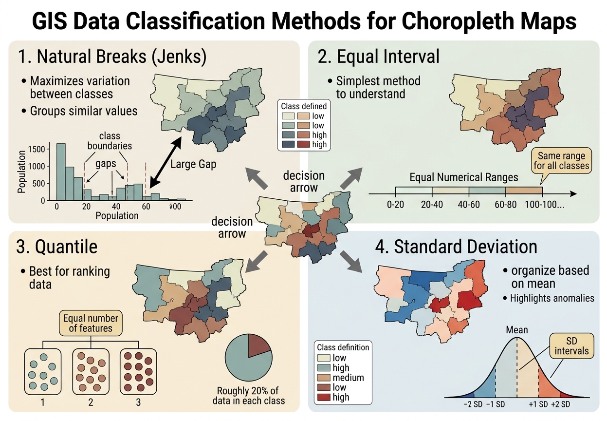
Data Classification Methods in GIS: Natural Breaks vs Equal Interval and Other Choropleth Methods

A choropleth map can make the same dataset tell very different visual stories depending on how numerical values are divided into classes. Data classification methods in GIS determine which observations are grouped together and therefore which areas appear “low,” “medium,” or “high” on the final map.

For GIS students, this is important because classification is not merely a formatting choice. A poor classification method can hide important variation, exaggerate differences, or create a misleading visual impression.

The four methods most commonly encountered in introductory GIS are:

Natural Breaks (Jenks)
Equal Interval
Quantile
Standard Deviation

Mastering these data classification methods in GIS prevents misinterpretation of spatial trends across choropleth maps.

1. Natural Breaks (Jenks)

Natural Breaks, also called Jenks Natural Breaks, attempts to place class boundaries where there are relatively large gaps in the data. When analyzing spatial data, choosing the right data classification methods in GIS helps highlight cluster patterns. Comparing different data classification methods in GIS helps analysts determine whether Jenks natural breaks best represent internal data groupings.

How it works

The algorithm searches for class boundaries that:

Minimize variation within each class
Maximize variation between classes

Imagine population values such as:

2, 3, 4, 5, 6, 8, 40, 45, 48, 52

There is a substantial gap between 8 and 40. Natural Breaks can recognize this separation and place a class boundary around it.

Best uses

Natural Breaks is particularly useful when:

Data are skewed
Values form recognizable clusters
There are natural gaps between groups
You want classes that reflect the structure of the dataset

It is commonly useful for mapping:

Population
Property values
Crime counts
Income
Disease cases
Other unevenly distributed socioeconomic data

Advantages

Reflects the actual distribution of the data
Can reveal meaningful clusters
Often produces visually intuitive maps
Useful for highly uneven datasets

Disadvantages

Class boundaries depend on the particular dataset
Two different datasets may produce completely different intervals
Comparisons between maps can become difficult
It may create classes with very unequal numerical ranges

Key idea: Natural Breaks asks, “Where does the data naturally separate?”

2. Equal Interval

Equal Interval divides the entire range of values into intervals of identical numerical width. When comparing spatial datasets, using standard data classification methods in GIS like Equal Interval keeps numerical ranges consistent.When reporting continuous spatial variables, standard data classification methods in GIS provide structured bounds for comparative reporting.

For example, suppose values range from 0 to 100 and you want five classes:

Class	Range
1	0–20
2	20–40
3	40–60
4	60–80
5	80–100

Every class covers exactly 20 units.

How it works

The calculation is essentially:

$Class interval=Maximum−MinimumNumber of classes\text{Class interval} = \frac{\text{Maximum}-\text{Minimum}}{\text{Number of classes}}$

Best uses

Equal Interval works well when:

The data are relatively uniformly distributed
The numerical range has meaningful interpretation
You want the map reader to understand the magnitude of values
The same class boundaries need to be applied consistently

It can be useful for variables such as:

Temperature
Rainfall
Elevation
Environmental measurements

Advantages

Very easy to understand
Class ranges have clear numerical meaning
Useful for comparing maps when identical intervals are retained
Simple to explain in an academic report

Disadvantages

If most observations are concentrated in a small part of the range, Equal Interval can produce classes containing very few or even no features.

For example, if most counties have populations between 0 and 30, but one city has a population of 100, several equal intervals may be dominated by that extreme value.

Key idea: Equal Interval asks, “How can I divide the numerical range into equal-sized pieces?”

3. Quantile Classification

Quantile classification creates classes containing approximately the same number of observations. When evaluating socioeconomic datasets, applying data classification methods in GIS such as Quantile helps rank geographic features into balanced categories.

For example, with 100 geographic features and five classes, each class would contain approximately 20 features.

The numerical ranges themselves may be very different.

Example

Suppose five classes are required:

Class	Number of areas
Very Low	20
Low	20
Moderate	20
High	20
Very High	20

The first class might cover a numerical range of only 0–10, while another could cover 10–100 if the data are highly skewed.

Best uses

Quantile works well when:

You want each class to contain a similar number of geographic units
You need strong visual differentiation across areas
The objective is to rank observations
The data distribution allows reasonably meaningful quantile groups

It can be useful for:

Socioeconomic rankings
Population comparisons
Election participation rates
Income rankings
Index scores

Advantages

Usually produces a visually balanced map
Makes it easy to distinguish high- and low-ranking areas
Avoids classes containing very few observations
Useful when relative ranking is more important than absolute magnitude

Disadvantages

Quantile can exaggerate small numerical differences.

For example, values of:

48, 49, 50, 51

might be placed into different classes simply because the method needs to distribute observations evenly.

Conversely, very different values might be grouped into the same class.

Key idea: Quantile asks, “How can I divide the observations into similarly sized groups?”

4. Standard Deviation

Standard Deviation classification organizes values according to their distance from the mean. Selecting appropriate data classification methods in GIS ensures outlier values stand out clearly against regional averages.

genui{“learning_viz”:{“type_id”:”STANDARD_DEVIATION”,”initial_values”:{“sigma”:1.5}}}

Instead of focusing primarily on the minimum and maximum values, the method emphasizes whether observations are:

Below the mean
Near the mean
Above the mean
Far from the mean

A map might therefore contain categories such as:

More than 2 standard deviations below the mean
1–2 standard deviations below the mean
Within 1 standard deviation of the mean
1–2 standard deviations above the mean
More than 2 standard deviations above the mean

Best uses

Standard Deviation is particularly useful when:

The mean is meaningful
The data have a reasonably symmetric distribution
You want to identify unusually high or low values
The objective is to show deviation from an average

Potential applications include:

Income relative to a regional mean
Rainfall anomalies
Population density deviations
Temperature anomalies
Crime rates relative to an average

Advantages

Highlights unusually high and low values
Provides statistical context
Useful for identifying areas that depart substantially from the mean
Particularly informative for approximately normally distributed data

Disadvantages

Less intuitive for audiences unfamiliar with standard deviation
Can work poorly with strongly skewed data
Class boundaries may not correspond to meaningful real-world thresholds

Key idea: Standard Deviation asks, “How unusual is this value compared with the dataset’s mean?”

Quick Reference Matrix

Classification Method	Best Data Type	Main Strength	Potential Visual Distortion
Natural Breaks (Jenks)	Skewed / clustered	Reveals natural groupings	Makes comparisons between different maps difficult
Equal Interval	Uniform / relatively even	Easy numerical interpretation	Can leave some classes nearly empty
Quantile	Ranked data / moderately distributed	Equal number of observations per class	Can exaggerate small differences
Standard Deviation	Normal / approximately symmetric	Shows deviation from mean	Can be misleading with highly skewed data

Important: “Best data type” is a guideline, not a rigid rule. The appropriate classification depends on the purpose of the map, the distribution of the data, and the intended audience.

Why Classification Can Change the Visual Story

Imagine two neighborhoods with values of 49 and 51.

With one classification method, both may appear in the same class.

With another, they could fall into different classes and receive noticeably different colors.

Now imagine two other neighborhoods with values of 10 and 30. A different classification could place both into the same category.

This demonstrates an important cartographic principle:

The map does not simply display the data; the classification system determines how the data are visually grouped.

Therefore, a GIS analyst should avoid choosing a classification method merely because it produces the most attractive map.

Practical Recommendation: Inspect the Histogram First

Before selecting a classification method in ArcGIS Pro or QGIS, examine the distribution of the variable.Understanding different data classification methods in GIS allows you to choose the right data representation for your audience.

Look for:

1. Clusters

If the histogram shows distinct groups separated by gaps, Natural Breaks may be appropriate.

2. A relatively even distribution

If values are spread relatively evenly across the range, Equal Interval may work well.

3. Strong ranking requirements

If you need approximately equal numbers of areas in each category, consider Quantile.

4. A meaningful mean

If the research question concerns how much areas deviate from the average, consider Standard Deviation.

5. Extreme skewness or outliers

Be cautious. An extreme value can strongly influence methods based on the minimum and maximum range.

In QGIS

When styling a graduated layer, inspect the distribution of your attribute values before settling on a classification. QGIS provides classification options including:

Equal Interval
Quantile
Natural Breaks (Jenks)
Standard Deviation
Pretty Breaks

Compare the resulting class boundaries and inspect how many features fall into each class. Experimenting with different data classification methods in GIS inside the layer style properties ensures your map effectively communicates spatial patterns.

In ArcGIS Pro

The Symbology pane’s graduated-colour classification tools allow you to compare classification methods and examine class breaks. Use the histogram to understand the distribution before deciding which classification communicates your variable appropriately. Comparing different data classification methods in GIS within the Symbology pane allows you to see how class breaks affect your map layout.

A Simple Decision Guide

Use this as a starting point:

Are there obvious clusters or gaps?
→ Consider Natural Breaks

Do you need equal numerical ranges?
→ Consider Equal Interval

Do you need roughly equal numbers of areas in each class?
→ Consider Quantile

Do you want to emphasize departures from the average?
→ Consider Standard Deviation

But always return to the research question.

For an academic GIS project, your report should ideally explain why you selected the classification method.

For example:

Natural Breaks (Jenks) classification was selected because the population values exhibited several distinct clusters, allowing the class boundaries to reflect the underlying distribution of the data.

That is considerably stronger than:

Natural Breaks was used because it looked better.

Final takeaway

There is no universally “best” data classification method in GIS. Natural Breaks, Equal Interval, Quantile, and Standard Deviation each emphasize different characteristics of the same dataset.Mastering these data classification methods in GIS ensures your choropleth maps remain accurate and unbiased.

Inspect the data distribution first, identify what you want the map to communicate, select an appropriate classification, and document that decision in your methodology.