Table of Contents

How to Use LiDAR Data in GIS: DEM, DSM & CHM

Introduction:What Is LiDAR Point Cloud Data and How to Use LiDAR Data in GIS

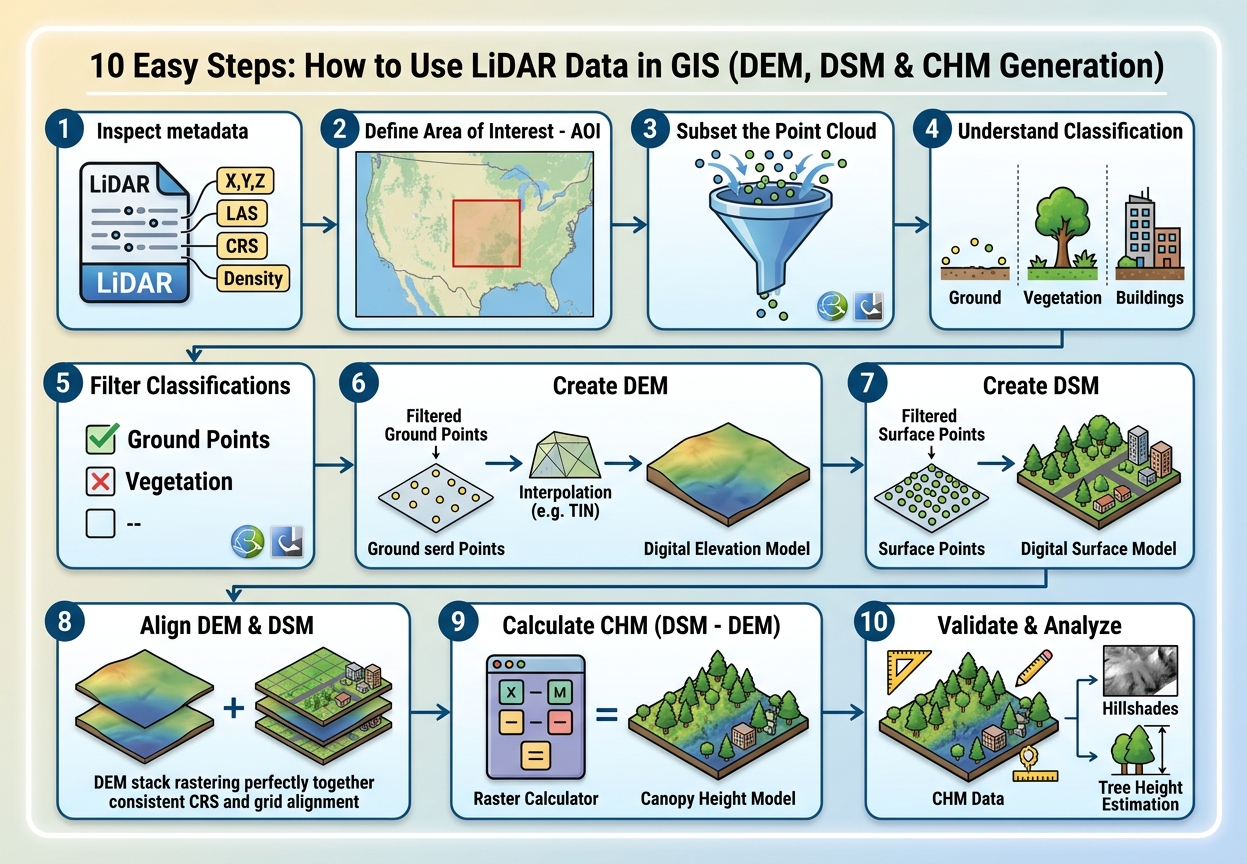
LiDAR data is a collection of millions of three-dimensional points captured by measuring the time it takes for laser pulses to travel from a sensor to the Earth’s surface and return. These points are commonly distributed in LAS or LAZ point-cloud files, which contain information such as X, Y, Z coordinates, return information, and point classification .In this step-by-step guide, we will cover how to use LiDAR data in GIS to generate DEM, DSM, and CHM rasters.

LiDAR is particularly valuable in GIS because it can capture detailed information about terrain, buildings, vegetation, and other objects above the ground. From the same point cloud, analysts can produce products such as a Digital Elevation Model (DEM), Digital Surface Model (DSM), and Canopy Height Model (CHM).

However, learning how to use LiDAR data in GIS introduces a common problem for students: LiDAR files can be extremely large. A single dataset can contain millions or even billions of points, making inefficient processing a frequent source of crashes, slow rendering, and failed remote sensing GIS assignment workflows.

The solution is not necessarily a more powerful computer. Good LiDAR processing begins with understanding point classifications, filtering, spatial resolution, and appropriate rasterization methods.

1.Understanding LiDAR Point Cloud Classification: How to Use LiDAR Data in GIS

Before creating a DEM or DSM, you need to understand what the individual points represent.

A LiDAR point cloud is not simply a collection of elevation measurements. Points can represent different objects depending on where the laser pulse was reflected.

Common LAS classification codes include:

Classification	Typical meaning
1	Unclassified
2	Ground
3	Low vegetation
4	Medium vegetation
5	High vegetation
6	Building
7	Low point/noise
8	Model key point
9	Water
17	Bridge deck

The exact classes available can vary depending on the LiDAR provider and processing specification, so always check the metadata accompanying your dataset.

Ground Points

Ground points are the most important points when creating a Digital Elevation Model.

Imagine a forested landscape:

        Trees
      /\/\/\/\/\
     /\/\/\/\/\/\
--------------------- Vegetation
       • • •
  •  •    •   •
_____________________ Ground

The ground-classified points represent the Earth’s terrain beneath vegetation and structures.

For a DEM, you generally want to work primarily with these points.

Vegetation Classes

Vegetation can be divided into several height categories.

Low vegetation

Examples include:

Grass
Small shrubs
Crops

Medium vegetation

Examples include:

Bushes
Young trees
Medium-height vegetation

High vegetation

Examples include:

Mature trees
Tall forest canopy

These classifications become particularly important when creating a Canopy Height Model.

Building Points

Building-classified points represent structures detected by the LiDAR classification process.

They are useful when creating a DSM because buildings are part of the surface visible to the sensor.

They may also be excluded when your analysis specifically requires vegetation or bare-earth elevation.

2. DEM vs DSM vs CHM

Three terms appear repeatedly when working with LiDAR:

DEM, DSM, and CHM.

Understanding their differences is essential before beginning your processing workflow.

What Is a Digital Elevation Model?

A Digital Elevation Model (DEM) represents the elevation of the bare-earth or ground surface.

Ideally, buildings, trees, and other above-ground objects have been removed.

For example:

Trees          Buildings
  /\              /\
 /  \      []    /  \
/    \____[]____/    \
________________________
        Ground

The DEM attempts to represent the line underneath the objects.

Ground-classified LiDAR points are therefore commonly used to generate a DEM.

Common DEM applications

DEM data can support:

Slope analysis
Aspect analysis
Watershed delineation
Flood modeling
Drainage analysis
Contour generation
Terrain visualization
Road planning

What Is a Digital Surface Model?

A Digital Surface Model (DSM) represents the elevation of the upper surface, including objects such as:

Trees
Buildings
Bridges
Other structures

Conceptually:

       Tree              Building
        /\                  ___
       /  \                |   |
______/    \_______________|   |____

The DSM therefore represents the top of features, rather than only the underlying terrain.

Depending on the dataset and processing method, DSM creation may use first returns or an appropriately filtered collection of non-ground points.

What Is a Canopy Height Model?

A Canopy Height Model (CHM) estimates vegetation height above the ground.

A common approach is:

$CHM=DSM-DEMCHM = DSM - DEM$

For example:

DSM elevation = 145 m
DEM elevation = 120 m

CHM = 145 - 120
CHM = 25 m

The result indicates that the feature’s surface is approximately 25 metres above the ground.

The concept is particularly useful for forestry.

A CHM can help identify:

Tree height
Canopy structure
Forest gaps
Vegetation density
Forest disturbance
Individual tree characteristics

However, interpretation depends on how the DSM and DEM were generated and how well the underlying point cloud represents the vegetation.

3. Step-by-Step LiDAR Processing Workflow

A typical LAS LAZ point cloud QGIS workflow looks like this:

Inspect metadata → Load point cloud → Filter classifications → Create DEM → Create DSM → Calculate CHM → Inspect/validate results

Let’s walk through each stage.

Step 1: Inspect the LiDAR Dataset

Before importing a huge file into your GIS project, examine its metadata.When learning how to use LiDAR data in GIS, always check your dataset metadata first.

Look for:

File format
Number of points
Point density
Coordinate reference system
Elevation units
Classification information
Point spacing
Geographic extent
Acquisition date
Vertical datum, if available

This information helps determine what the dataset can realistically be used for.

For example, a dataset with high point density can support detailed terrain modeling, while a sparse dataset may require a coarser output resolution.

Step 2: Avoid Loading the Entire Dataset Unnecessarily

A common beginner mistake is opening a massive LiDAR file and immediately attempting to visualize or process every point.

If the dataset covers a large region, first define your Area of Interest (AOI).

For a university assignment, you may only need a few square kilometres.

Instead of processing:

Entire county
↓
Hundreds of millions of points

work with:

Study area
↓
AOI subset
↓
Relevant point classes
↓
Raster product

This can dramatically reduce processing requirements.

Step 3: Loading LAS/LAZ in QGIS

Modern QGIS versions can work with point-cloud data through native point-cloud support and appropriate providers.

A typical workflow is:

Open QGIS.
Use Layer → Add Layer → Add Point Cloud Layer.
Browse to your .las or .laz file.
Add the layer.
Inspect the point cloud visually.
Check the layer properties and CRS.

LAZ files are compressed versions of LAS data and are often preferable when storage space is limited.

If your computer struggles

Do not immediately assume the data is corrupt.

Try:

Working with a smaller AOI.
Using a spatial subset.
Processing only required classifications.
Reducing display density.
Creating raster derivatives rather than repeatedly rendering the full point cloud.

The key principle is:

Don’t process more points than your assignment requires.

Step 4: Loading LiDAR into ArcGIS Pro

ArcGIS Pro can also work with LAS/LAZ data through its LAS and point-cloud workflows.

A typical workflow involves:

Open ArcGIS Pro.
Create or open your project.
Add the LAS/LAZ data or create a LAS dataset where appropriate.
Inspect the point cloud.
Examine point classifications.
Define the processing extent.
Use the appropriate LAS/raster conversion tools to generate elevation surfaces.

For larger projects, working through a LAS dataset can help organize multiple LiDAR files rather than treating every file independently.

Step 5: Filter Points by Classification

This is where the point cloud becomes useful for modeling.

Creating a DEM

For a basic bare-earth DEM:

Select ground points.

Conceptually:

LAS/LAZ
   ↓
Classification filter
   ↓
Ground (Class 2)
   ↓
Interpolation
   ↓
DEM

This removes trees and buildings from the terrain model as long as the classification is accurate.

Creating a DSM

For a DSM, you want points representing the surface features.

Depending on the dataset and desired methodology, this can include:

Vegetation
Buildings
Other above-ground features

A simplified workflow is:

LAS/LAZ
   ↓
Surface/non-ground points
   ↓
Rasterization/interpolation
   ↓
DSM

Be careful with the phrase “first return = DSM.” First returns can be useful for representing elevated surfaces, but they are not automatically equivalent to a clean DSM. The correct approach depends on the point-cloud characteristics and the software workflow being used.

Step 6: Interpolate the Point Cloud into a Raster

A point cloud consists of discrete points.

A DEM or DSM is normally represented as a continuous raster surface.

You therefore need a method to transform point elevations into raster cells.

Two commonly encountered approaches are IDW and TIN. Interpolation is a crucial step when you learn how to use LiDAR data in GIS applications.

IDW Interpolation

A Triangulated Irregular Network (TIN) represents the su

Inverse Distance Weighted (IDW) estimates the value of an unknown location based on nearby known points.

The basic idea is:

Nearby points have greater influence than distant points.

For example, if a raster cell is surrounded by several LiDAR points, the closest points contribute more strongly to the estimated elevation.

IDW can be useful for relatively straightforward surfaces, but its suitability depends on point distribution and terrain characteristics.

TIN Interpolationrface using interconnected triangles.

Conceptually:

     •---------•
      \       / \
       \     /   \
        \   /     •
         \ /
          •

Each triangle describes part of the surface.

TINs can preserve terrain structure effectively, particularly where the input points are unevenly distributed.

For LiDAR processing, however, the most appropriate interpolation/rasterization method depends on your software, point density, terrain, required accuracy, and assignment methodology. Some LiDAR-specific tools use methods beyond simple IDW or TIN.

Step 7: Choose an Appropriate Raster Resolution

One of the most important decisions in Digital Elevation Model creation is choosing the output cell size.

Suppose your LiDAR data has an average point spacing of approximately 1 metre.

You might produce:

1 m DEM

But that does not automatically mean a 1 m DEM is the correct choice for every assignment.

A very fine raster:

Contains more cells
Requires more storage
Takes longer to process
May expose noise
Can exceed what the data density supports

A very coarse raster:

Processes faster
Uses less storage
May smooth important terrain features
Can lose detail

Choose a resolution based on:

Point density
Intended analysis
Study-area size
Required accuracy
Computing resources

Your methodology should explain why you selected the chosen resolution.

Step 8: Create the DEM

The simplified DEM workflow is:

Ground-classified points
          ↓
Filter
          ↓
Interpolate/rasterize elevation
          ↓
DEM

After creating the DEM, inspect it visually.

You can derive:

Hillshade
Slope
Aspect
Contours
Flow direction
Flow accumulation

These derivatives are useful for terrain and hydrological analysis.

Step 9: Create the DSM

The DSM workflow is similar:

Surface points
      ↓
Filter/select appropriate returns
      ↓
Rasterize/interpolate
      ↓
DSM

Inspect the resulting surface.

Trees should appear as elevated features, while buildings should also be visible where the point cloud captures them.

Step 10: Create the Canopy Height Model

Once the DEM and DSM have been created and aligned, calculate:

$CHM=DSM-DEMCHM = DSM - DEM$

In a raster calculator, the conceptual operation is:

DSM - DEM

For example:

Location	DSM	DEM	CHM
Forest A	142 m	118 m	24 m
Forest B	136 m	120 m	16 m
Open ground	121 m	120 m	1 m

Areas where DSM and DEM are nearly equal represent surfaces close to ground level.

Areas with large differences indicate elevated features.

4. Troubleshooting Common LiDAR Problems

Problem 1: The LAS/LAZ File Is Too Large

This is probably the most common student problem.

Symptoms include:

QGIS becomes unresponsive.
ArcGIS Pro takes a long time to draw.
Processing appears frozen.
Your computer runs out of memory.
Raster generation takes excessively long.

Solution

Reduce the workload.

Use:

An AOI
Classification filtering
Spatial subsets
Appropriate raster resolution
Smaller processing tiles

If your assignment covers a 5 km² study area, there is little reason to process hundreds of square kilometres of LiDAR data.

Problem 2: Your Point Cloud Has Few or No Classified Points

You may open a dataset and discover that most points are classified as Unclassified (Class 1).

This creates a problem if your workflow specifically requires ground points.

For example:

Required:
Class 2 = Ground

Available:
Class 1 = Unclassified

Simply filtering for Class 2 could therefore produce an empty or incomplete dataset.

Solution

Check the metadata and dataset documentation.

Determine whether:

The dataset genuinely has no classification.
Classification exists but uses a different scheme.
The software is interpreting the classification incorrectly.
Ground classification needs to be performed separately.

Do not arbitrarily assume that Class 1 means ground.

Problem 3: DEM Contains Trees and Buildings

If your supposed bare-earth DEM contains obvious buildings or tree elevations, your input filtering is probably incorrect.

Check:

Point classification
Ground filtering
Interpolation settings
Outliers
NoData areas

A DEM should represent the terrain rather than the tops of trees and buildings.

Problem 4: CHM Contains Negative Values

A CHM is commonly calculated as:

DSM - DEM

You may occasionally find negative values.

Possible causes include:

DEM and DSM generated using inconsistent methods
Misalignment
Different vertical references
Interpolation artifacts
Classification errors
Noise

Do not automatically delete negative values without investigating why they occurred.

Problem 5: DEM and DSM Don’t Line Up

Before calculating:

DSM - DEM

both rasters need compatible:

CRS
Cell size
Extent
Grid alignment

Otherwise, raster subtraction can produce incorrect results or require resampling.

LiDAR Applications in Remote Sensing and GIS

LiDAR is useful far beyond simply producing an elevation map.

Forestry

A CHM can support:

Tree-height estimation
Canopy structure analysis
Forest inventory
Biomass estimation
Forest disturbance mapping
Individual-tree detection

For example, a forest manager could use a CHM to identify areas containing unusually tall or dense vegetation.

Flood Risk Modeling

A high-resolution DEM can provide detailed information about terrain elevation.

This can support:

Drainage analysis
Flow accumulation
Watershed delineation
Floodplain mapping
Terrain-based flood modeling

Small changes in elevation can significantly affect modeled drainage pathways, particularly in relatively flat environments.

Urban Analysis

LiDAR-derived DSMs can also support:

Building-height analysis
3D city modeling
Urban morphology
Visibility studies
Solar potential analysis

A Practical LiDAR Workflow for a GIS Assignment

For an introductory remote sensing project, the entire workflow can be summarized as:

        LAS / LAZ
            ↓
     Inspect metadata
            ↓
       Define AOI
            ↓
      Filter points
       ↙          ↘
   Ground        Surface
     ↓               ↓
   DEM              DSM
      \              /
       \            /
        └── DSM-DEM ┘
              ↓
             CHM
              ↓
     Analysis + Mapping

Keep a record of every important processing decision:

Processing stage	Record
Dataset	LAS/LAZ source
CRS	Horizontal/vertical reference
AOI	Study-area boundary
Filter	Point classifications/returns
DEM method	Interpolation/rasterization
DSM method	Interpolation/rasterization
Resolution	Cell size
CHM	DSM − DEM
Validation	Visual/quantitative checks

This documentation can make the difference between simply producing a map and producing a defensible remote sensing GIS assignment.

Conclusion

Learning how to use LiDAR data in GIS starts with understanding that a point cloud contains much more information than a collection of elevation points.

The essential workflow is:

Inspect → subset → classify/filter → rasterize → validate → analyze.

Remember the fundamental distinction:

DEM → ground/bare-earth elevation
DSM → elevation of the surface, including above-ground features
CHM → relative vegetation/object height, commonly calculated as DSM − DEM

For students, the biggest practical challenges are usually large LAS/LAZ files, unsuitable raster resolutions, inconsistent coordinate systems, and unclassified points. Handling these issues systematically makes LiDAR processing much more manageable.In this step-by-step guide, we will cover how to use LiDAR data in GIS to generate DEM, DSM, and CHM rasters.In this step-by-step guide, we will cover how to use LiDAR data in GIS to generate DEM, DSM, and CHM rasters.

Once you can turn a LiDAR point cloud into reliable DEM, DSM, and CHM products, you have a foundation for more advanced GIS and remote-sensing applications—including forest structure analysis, terrain modeling, flood-risk assessment, hydrology, urban analysis, and 3D environmental modeling.