
Building a Serverless Spatial Data Lakehouse with GeoParquet, Apache Iceberg, and DuckDB
Introduction
When building a Serverless Spatial Data Lakehouse GeoParquet DuckDB stack, geospatial data engineering is increasingly concerned with datasets too large, too frequently updated, or too geographically distributed for conventional database architectures to handle efficiently. Geospatial data engineering is increasingly concerned with datasets too large, too frequently updated, or too geographically distributed for conventional database architectures to handle efficiently. Satellite imagery footprints, mobility trajectories, road networks, environmental observations, and cadastral records can collectively reach billions of features and terabytes or petabytes of analytical data.
Traditional spatial databases such as PostgreSQL with PostGIS remain valuable for transactional applications, indexed feature retrieval, and operational GIS. However, scaling them for predominantly analytical workloads can introduce substantial storage, index-maintenance, compute-provisioning, and infrastructure-management costs. Large spatial joins, historical comparisons, and repeated full-dataset aggregations can also compete with latency-sensitive application queries.
A modern data stack geospatial analytics architecture separates durable storage from query execution. Instead of loading every feature into a continuously running database server, engineers store compressed, columnar data in object storage and execute analytical jobs against only the necessary files, columns, and row groups.
Three technologies are particularly useful in this design:
-
Amazon S3 supplies durable, scalable object storage for spatial data and table metadata.
-
Apache Iceberg provides open table management, snapshots, schema evolution, partition evolution, and transactional commits.
-
DuckDB supplies an embedded analytical SQL engine that can execute spatial queries directly against remote data.
GeoParquet complements these components by standardizing how geometry columns and their geospatial metadata are represented in Parquet files. Its current 2.0 specification uses Parquet’s native GEOMETRY and GEOGRAPHY logical types, although compatibility must be checked across the specific writers and readers in a deployment.
The resulting architecture is a serverless spatial data lakehouse using GeoParquet, Apache Iceberg, and DuckDB: data remains in inexpensive object storage, table state is governed by an open format, and compute can be provisioned for individual analytical jobs.
The important architectural distinction is that serverless describes how compute is deployed, not an intrinsic property of DuckDB. DuckDB is an embedded engine that can run inside short-lived workers or managed compute environments rather than requiring a continuously running database cluster.
1. Architecture and Component Stack for a Serverless Spatial Data Lakehouse GeoParquet DuckDB
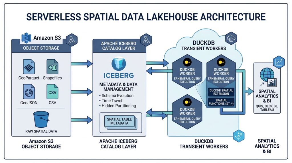
The reference architecture consists of a storage layer, an open table-format layer, and an analytical execution layer.
[Image 1: Architecture diagram of a serverless spatial data lakehouse connecting S3, Iceberg, and DuckDB]
Alt text: “System architecture diagram illustrating a serverless spatial data lakehouse processing GeoParquet files stored in S3 via Apache Iceberg catalogs and DuckDB compute.”
1.1 Amazon S3: The storage foundation
S3 stores the Parquet data files and the supporting Iceberg metadata. Separate prefixes can hold raw ingestion files, validated GeoParquet datasets, and table-managed analytical data.
A practical layout might look like this:
s3://geo-lake/
├── raw/
│   └── asset_observations/
├── staging/
│   └── asset_observations/
└── warehouse/
    └── asset_observations/
        ├── data/
        └── metadata/
The staging area contains validated input files awaiting ingestion. The warehouse prefix contains files managed through Iceberg commits, together with metadata and snapshot manifests.
This distinction matters because uploading a Parquet file into a directory does not automatically make it part of an Iceberg table. Iceberg tracks which files belong to each committed table snapshot. Unmanaged objects can exist alongside a table without becoming visible through its catalog entry.
DuckDB’s httpfs extension supports remote object storage access through the S3 API, including reading selected byte ranges rather than downloading every complete file. Its AWS integration can also provide credential-chain authentication.
1.2 Apache Iceberg: Table state and transactional consistency
Apache Iceberg sits between physical storage and analytical clients. Instead of treating an S3 prefix as a complete table, Iceberg maintains metadata identifying the current schema, partition specifications, snapshots, manifests, and data files.
When a writer publishes a successful commit, it updates the table metadata reference. Readers can therefore use a consistent snapshot even while new versions are being committed. Historical snapshots can be retained for time-travel queries, subject to the table’s snapshot-retention policy.
For spatial data engineering, Iceberg provides several important capabilities:
-
Atomic publication of newly ingested or transformed datasets.
-
Snapshot-based reproducibility for historical spatial analysis.
-
Schema evolution without necessarily rewriting existing data files.
-
Partition evolution as data volumes and query patterns change.
-
Catalog-based discovery across compatible analytical engines.
Iceberg is not, by itself, a spatial database. It does not automatically provide a PostGIS-style spatial index or guarantee that a polygon-intersection query will prune every irrelevant file. Spatial performance still depends on partition design, file statistics, physical data layout, and query predicates.
1.3 DuckDB: Ephemeral analytical compute
DuckDB executes SQL against Iceberg tables and Parquet data. Its spatial functions support operations such as intersections, spatial aggregations, coordinate transformations, and bounding-box predicates.
The iceberg extension supports reading individual tables from their metadata and accessing catalog-managed tables through an Iceberg REST catalog. Direct metadata-path access is read-only; catalog attachment is required for the documented catalog-managed write workflow.
For a serverless deployment, DuckDB can run in an ephemeral Python worker launched by an event-driven service, scheduled workflow, or managed container task. Each job authenticates to the object store, resolves the table metadata, executes its SQL, writes results, and terminates.
This approach is suitable for bounded analytical jobs where a single worker can process the necessary data within its CPU, memory, execution-time, and network limits. A petabyte-scale lake does not imply that one DuckDB process can scan petabytes efficiently; distributed engines remain appropriate when parallel compute capacity exceeds a single worker’s practical limits.
1.4 The end-to-end query path
A well-designed query follows this sequence:
-
DuckDB resolves the requested Iceberg table through its catalog.
-
Iceberg metadata identifies candidate data files and their partition and file-level statistics.
-
Parquet scanning reads only the required columns and can skip irrelevant row groups where statistics support the filters.
-
Spatial bounding-box predicates reduce the candidate geometry records.
-
Exact spatial predicates perform the required topological tests.
-
DuckDB aggregates the surviving records and returns or persists the results.
Each stage eliminates work before the next stage becomes expensive. This is the central principle behind efficient cloud spatial analytics.
2. Step One: Structure and Partition GeoParquet Data in S3
The first implementation decision is how to transform source GIS data into a columnar layout that supports efficient cloud queries.
Simply converting a Shapefile or GeoPackage into Parquet is insufficient for a large lakehouse. The pipeline must establish a consistent geometry representation, coordinate reference system (CRS), schema, spatial ordering strategy, and file-partitioning policy.
2.1 Establish a consistent spatial schema
Consider an asset-observation dataset containing building footprints, inspection dates, asset identifiers, and source geometry.
A suitable logical schema is:
| Column | Type | Purpose |
|---|---|---|
asset_id |
BIGINT |
Stable feature identifier |
event_time |
TIMESTAMP |
Observation timestamp |
tile_id |
VARCHAR |
Derived spatial tile identifier |
geom |
GEOMETRY |
Feature geometry |
xmin, ymin |
DOUBLE |
Lower bounding-box coordinates |
xmax, ymax |
DOUBLE |
Upper bounding-box coordinates |
The explicit bounding-box columns are useful for a compatibility-oriented implementation because they allow ordinary numeric filters to reach Parquet’s statistics-based pruning mechanisms. They are not mandatory GeoParquet fields in every specification version.
Before writing, standardize the CRS and verify that the geometry column contains valid geometries of the expected types. The example below uses geographic coordinates in longitude-latitude order. For planar measurements, reproject into a suitable projected CRS rather than assuming longitude and latitude represent linear distances.
2.2 Write partition-sized batches
Use GeoPandas for a manageable ingestion batch, and stage the results in S3. For a very large dataset, execute the same operation in bounded batches instead of materializing the full dataset in memory.
import geopandas as gpdimport pandas as pd# Example: one batch of source features.gdf = gpd.read_file("input_assets.gpkg")# Establish a consistent geographic CRS.gdf = gdf.to_crs("OGC:CRS84")# Derive scalar spatial-filtering columns.bounds = gdf.geometry.boundsgdf["xmin"] = bounds["minx"]gdf["ymin"] = bounds["miny"]gdf["xmax"] = bounds["maxx"]gdf["ymax"] = bounds["maxy"]# Keep event timestamps consistently typed.gdf["event_time"] = pd.to_datetime( gdf["event_time"], utc=True)# tile_id should be generated by a consistent# tiling scheme in the upstream processing pipeline.assert gdf["tile_id"].notna().all()# Write a staged columnar batch.gdf.to_parquet( "asset_batch.parquet", compression="zstd", index=False,)This example uses a single local staging file. The production pipeline should upload each completed batch to a unique S3 staging key, using an appropriate S3 client or filesystem integration.
GeoParquet provides geometry metadata alongside the columnar file structure, allowing compatible readers to interpret the geometry column and its CRS. Verify the resulting metadata rather than assuming every Parquet writer produces the same GeoParquet specification version.
For the underlying cloud-reading pattern, see Querying GeoParquet Files Directly from Amazon S3 Using DuckDB and Python.
2.3 Design partitions around query patterns
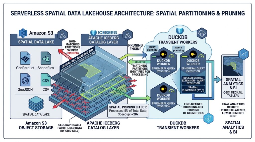
Partitioning is not simply a matter of splitting data into folders. It determines how much data an analytical engine must consider before it can execute a query.
A useful initial strategy combines a temporal dimension with a derived spatial identifier. For example, a table could be partitioned by observation month and a bounded number of hash buckets over tile_id.
CREATE TABLE lake.geo.asset_observations (
    asset_id BIGINT,
    event_time TIMESTAMP,
    tile_id VARCHAR,
    geom GEOMETRY,
    xmin DOUBLE,
    ymin DOUBLE,
    xmax DOUBLE,
    ymax DOUBLE
)
PARTITIONED BY (
    month(event_time),
    bucket(32, tile_id)
);
This is an Iceberg table definition, not an S3 directory-creation command. The catalog and writer manage the resulting data layout.
The bucket transform distributes high-cardinality values across a bounded number of partitions. However, a bucket is not a geographic region: spatial filtering must still identify candidate tile IDs and apply geometry-level predicates.
Avoid using raw longitude and latitude as unbounded partition dimensions. Likewise, partitioning by individual feature IDs can generate excessive small partitions. Iceberg supports multiple partition transforms and partition evolution, so the design can change as workload characteristics develop.
For raster-oriented pipelines, a complementary preprocessing approach is described in Optimizing Raster Processing Performance with GDAL Multi-Threading and VRT Files.
3. Step Two: Register the Dataset with Apache Iceberg
Once staged GeoParquet files have passed validation, they must become part of a committed Iceberg table.
There are two common approaches:
Managed ingestion: Read the staged files and write their records into an Iceberg table. The writer creates the required data files and commits the table metadata.
Metadata-based file import: Where the chosen engine and catalog support it, import compatible existing Parquet files into an Iceberg table without rewriting their contents. This requires explicit validation of the existing schema, file metadata, and compatibility with every downstream reader.
For a DuckDB-centric implementation, catalog-managed ingestion provides a straightforward starting point.
3.1 Configure DuckDB and the catalog
Install the necessary extensions in the execution environment:
import duckdbcon = duckdb.connect()con.execute("INSTALL aws")con.execute("LOAD aws")con.execute("INSTALL httpfs")con.execute("LOAD httpfs")con.execute("INSTALL spatial")con.execute("LOAD spatial")con.execute("INSTALL iceberg")con.execute("LOAD iceberg")Use a temporary identity with narrowly scoped permissions to read the staging prefix, write the warehouse prefix, and access the catalog. Where available, use workload identity or a credential chain rather than embedding long-lived credentials in source code.
Configure S3 authentication:
CREATE SECRET s3_auth (
    TYPE s3,
    PROVIDER credential_chain,
    REGION 'us-east-1'
);
The region and credential provider must match the deployment.
Next, attach a compatible Iceberg REST catalog. This illustrative example uses OAuth2-style authentication; actual catalog endpoints and authentication options depend on the selected service.
CREATE SECRET iceberg_auth (
    TYPE iceberg,
    CLIENT_ID 'YOUR_CLIENT_ID',
    CLIENT_SECRET 'YOUR_CLIENT_SECRET',
    OAUTH2_SERVER_URI
        'https://catalog.example.com/v1/oauth/tokens'
);

ATTACH 'geo-warehouse' AS lake (
    TYPE iceberg,
    SECRET iceberg_auth,
    URI 'https://catalog.example.com'
);

CREATE SCHEMA lake.geo;
DuckDB documents REST-catalog attachment as the entry point for catalog-managed Iceberg operations, including table creation and writes.
3.2 Ingest validated files into the managed table
Create a partitioned destination table and insert the staged records:
CREATE TABLE lake.geo.asset_observations (
    asset_id BIGINT,
    event_time TIMESTAMP,
    tile_id VARCHAR,
    geom GEOMETRY,
    xmin DOUBLE,
    ymin DOUBLE,
    xmax DOUBLE,
    ymax DOUBLE
)
PARTITIONED BY (
    month(event_time),
    bucket(32, tile_id)
);

INSERT INTO lake.geo.asset_observations
SELECT
    asset_id,
    event_time,
    tile_id,
    geom,
    xmin,
    ymin,
    xmax,
    ymax
FROM read_parquet(
    's3://geo-lake/staging/asset_observations/*.parquet'
);
This is a minimal ingestion pattern: the source schema must match the destination types, and the actual S3 paths must resolve to validated staged files. Larger datasets should generally be ingested incrementally rather than through one enormous insert.
The Iceberg writer publishes the new table state through the catalog. Do not write files directly into the table’s managed data directory and assume that the catalog will discover them.
A production deployment must also test geometry serialization and round-trip compatibility across the exact DuckDB, Iceberg extension, GeoParquet writer, and downstream reader versions. DuckDB-Iceberg’s documented limitations include unsupported GEOGRAPHY table types, so the examples use GEOMETRY.
3.3 Validate snapshots and historical state
Iceberg snapshots enable engineers to audit changes and reproduce an earlier analytical view.
For example, DuckDB supports time-travel reads from an attached catalog:
SELECT COUNT(*)
FROM lake.geo.asset_observations
AT (
    TIMESTAMP =>
        TIMESTAMP '2026-10-01 00:00:00'
);
The timestamp must correspond to a retained historical table state. It is not a guarantee that arbitrary deleted objects remain available forever: snapshot expiration and file cleanup policies determine how long historical states can be queried.
This capability is particularly valuable for environmental monitoring, land-cover change analysis, asset inventories, and regulatory reporting, where results may need to be reproduced from a prior data publication.
4. Step Three: Execute Spatial Aggregations with Python and DuckDB
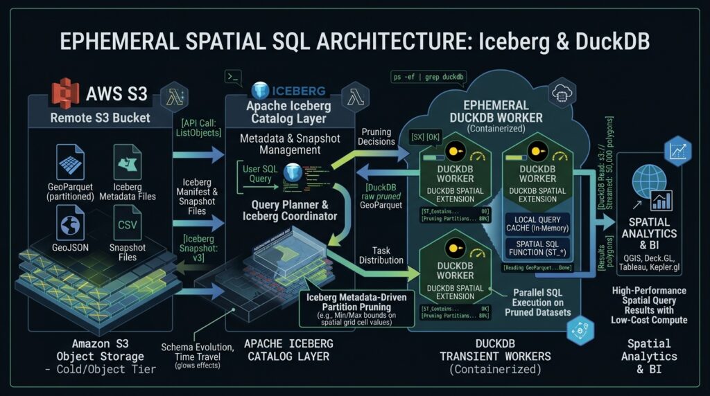
The analytical layer should be organized around repeatable, bounded query jobs. Each worker resolves its inputs, executes the required SQL, and exports a compact result rather than downloading an entire spatial dataset to Python.
The following example calculates the number of qualifying observations within an area of interest.
First, establish the catalog connection using the configuration described previously. Then run:
import duckdbcon = duckdb.connect()con.execute("INSTALL httpfs")con.execute("LOAD httpfs")con.execute("INSTALL spatial")con.execute("LOAD spatial")con.execute("INSTALL iceberg")con.execute("LOAD iceberg")# In production, configure the S3 secret and attach# the Iceberg REST catalog before querying.query = """SELECT tile_id, COUNT(*) AS observation_countFROM lake.geo.asset_observationsWHERE event_time >= TIMESTAMP '2026-01-01 00:00:00' AND event_time < TIMESTAMP '2026-02-01 00:00:00'GROUP BY tile_idORDER BY observation_count DESC"""result = con.execute(query).fetchdf()result.to_parquet( "monthly_tile_summary.parquet", index=False,)This example demonstrates temporal filtering and aggregation; it does not yet apply an area-of-interest geometry. The next section adds that filter.
4.1 Treat the execution environment as disposable
The query worker does not need persistent local storage for the underlying lakehouse. It can use temporary disk space for spill, buffering, and intermediate results, subject to the hosting platform’s limits.
A practical orchestration sequence is:
-
Receive a scheduled or event-driven query request.
-
Load credentials and attach the relevant catalog.
-
Execute SQL with bounded memory, execution time, and concurrency.
-
Write the analytical output to a results prefix or downstream table.
-
Record execution metrics and terminate the worker.
This provides operational isolation between jobs and avoids maintaining a dedicated cluster for intermittent workloads.
However, serverless orchestration does not eliminate the need for cost controls. Large spatial joins can generate substantial intermediate data, object-store requests, and temporary disk usage. Worker sizing and workload admission should be based on measured query performance.
For exceptionally large joins, sustained high concurrency, or complex distributed processing, use DuckDB as one component in a broader analytical platform rather than treating it as a replacement for every distributed query engine.
5. Step Four: Optimize Spatial Predicate Pushdown
Spatial performance often depends on how quickly a query eliminates candidate features before exact geometry calculations begin.
The key distinction is between a bounding-box test and an exact spatial predicate. A geometry may intersect an area’s bounding rectangle without intersecting the actual polygon.
5.1 Use bounding-box filters as the first stage
A robust predicate design combines inexpensive coordinate comparisons with an exact geometry test.
DuckDB provides ST_Intersects_Extent and the && bounding-box overlap operator; ST_Intersects evaluates the actual geometric intersection. Do not assume that ST_BBoxIntersectsis a native DuckDB function in your target version.
For example, suppose the query area is a polygon in the same CRS as the stored geometry:
WITH roi AS (
    SELECT ST_GeomFromText(
        'POLYGON((
            10 10, 20 10, 20 20,
            10 20, 10 10
        ))'
    ) AS geom
)
SELECT
    a.asset_id,
    a.tile_id
FROM lake.geo.asset_observations AS a
CROSS JOIN roi
WHERE a.xmin <= 20
  AND a.xmax >= 10
  AND a.ymin <= 20
  AND a.ymax >= 10
  AND ST_Intersects(a.geom, roi.geom);
The numeric conditions identify geometries whose bounding boxes overlap the region’s bounding box. The final ST_Intersects condition removes false positives.
The coordinate bounds in this example are illustrative. In production, calculate the region’s bounds from the query geometry and ensure they use the same CRS as the stored bounding-box columns. Handle antimeridian-crossing geometries and other CRS edge cases explicitly.
5.2 Understand where pushdown actually occurs
There are several distinct optimization layers:
| Optimization layer | What it can eliminate |
|---|---|
| Iceberg partition pruning | Partitions excluded by the query’s compatible scalar filters |
| Iceberg manifest and file statistics | Files whose recorded metadata proves they cannot match |
| Parquet statistics | Row groups or pages that cannot match supported column predicates |
| Bounding-box filtering | Features whose rectangular extents cannot intersect the query extent |
| Exact spatial evaluation | Geometries that fail the actual topological predicate |
These mechanisms complement one another, but they are not interchangeable.
GeoParquet’s current specification builds on Parquet’s native geospatial types and statistics. Compatibility-oriented pipelines may also store explicit bounding-box columns to expose ordinary numeric statistics to readers that do not exploit geometry statistics directly.
For dependable pruning, test the generated files and query plan on the production reader. Merely writing ST_Intersects_Extent in a WHERE clause does not guarantee that the expression will become an S3-level filter or cause every irrelevant row group to be skipped.
5.3 Improve physical data locality
If nearby geometries are scattered throughout every file, bounding-box filtering may still leave many candidate row groups.
Improve locality by ordering data using a consistent spatial index or curve, such as a tile identifier or Hilbert-derived spatial key, before writing reasonably sized files and row groups. The DuckDB spatial extension provides ST_Hilbert for deriving a Hilbert-curve index from spatial coordinates or bounding boxes.
Combine spatial locality with temporal organization when query workloads commonly filter by time and location. For example, monthly partitions can eliminate historical periods, while tile-based data organization improves candidate-file selection within each period.
Also avoid producing thousands of tiny files for small geographic tiles. File-open overhead, metadata planning, and excessive object-store requests can outweigh the benefit of finer spatial granularity.
The practical optimization target is not simply fewer geometry calculations. It is fewer files opened, fewer bytes transferred, fewer rows decoded, and fewer exact geometry operations per query.
6. Production Hardening and Enterprise Operations
A working prototype is not yet an enterprise lakehouse. Production readiness requires governance, observability, data-quality controls, and a maintenance strategy.
Schema and geometry validation. Validate geometry types, CRS metadata, null geometry handling, attribute types, and identifier uniqueness where required. Reject incompatible source batches before publication.
Snapshot and catalog management. Establish retention policies based on reproducibility requirements. Schedule the appropriate Iceberg maintenance operations, including snapshot expiration, orphan-file cleanup, and compaction where supported by the chosen catalog and maintenance engine.
File-layout management. Monitor file sizes, row-group sizes, compression, spatial ordering, and the distribution of rows across partitions. Revisit partition transforms when query selectivity or ingest volume changes substantially.
Access security. Use separate permissions for staging ingestion, table writes, and analytical reads. Protect catalog credentials, log the identity that executed each job, and avoid exposing unrestricted access to sensitive spatial records.
Observability. Record scanned bytes, output rows, execution duration, memory usage, spill volume, query failures, and object-store request counts. Benchmark representative queries before and after layout changes rather than assuming that a particular partitioning scheme is faster.
Interoperability testing. Validate that data remains readable by all required engines after changes to table schemas, geometry encodings, metadata versions, or writer versions. An open table format does not automatically guarantee that every engine implements every spatial extension identically.
Teams maintaining transactional application workloads may also benefit from Spatial Index Tuning and Database Partitioning Strategies for Billion-Row PostGIS Tables. PostGIS and an Iceberg lakehouse serve different workload profiles, and both can coexist in a modern data platform.
Summary and Enterprise Takeaways
A serverless spatial data lakehouse separates inexpensive durable storage from table management and analytical compute. GeoParquet supplies a portable columnar representation for geometry, Apache Iceberg manages table state and historical snapshots, and DuckDB enables SQL-based spatial analysis without requiring a permanently running database server.
The architecture succeeds when its components are designed together. Ingestion must produce valid, interoperable spatial data; Iceberg must manage committed files and metadata; and DuckDB queries must exploit partition pruning, Parquet statistics, bounding-box filters, and exact geometry predicates in the right order.
For enterprise deployments, the most important takeaways are:
-
Design for selective reads: Spatial locality, sensible file sizes, and reliable predicate pushdown matter more than simply putting Parquet files in S3.
-
Preserve transactional correctness: Use Iceberg-aware writers and catalog commits instead of treating warehouse prefixes as unmanaged folders.
-
Validate interoperability: Confirm that the chosen GeoParquet version, geometry types, catalog, and query engines work together.
-
Scale compute according to the workload: Short-lived DuckDB workers are effective for bounded analytical jobs, but extremely large or highly concurrent workloads may require distributed execution.
-
Measure the entire pipeline: Optimize data preparation, metadata planning, bytes scanned, geometry processing, and operational costs together.
The resulting platform provides an open, modular foundation for cloud-native geospatial analytics without forcing every workload into a permanently provisioned spatial database. Its long-term value comes from combining portable data formats, transactional table management, selective analytical execution, and disciplined operational practices.