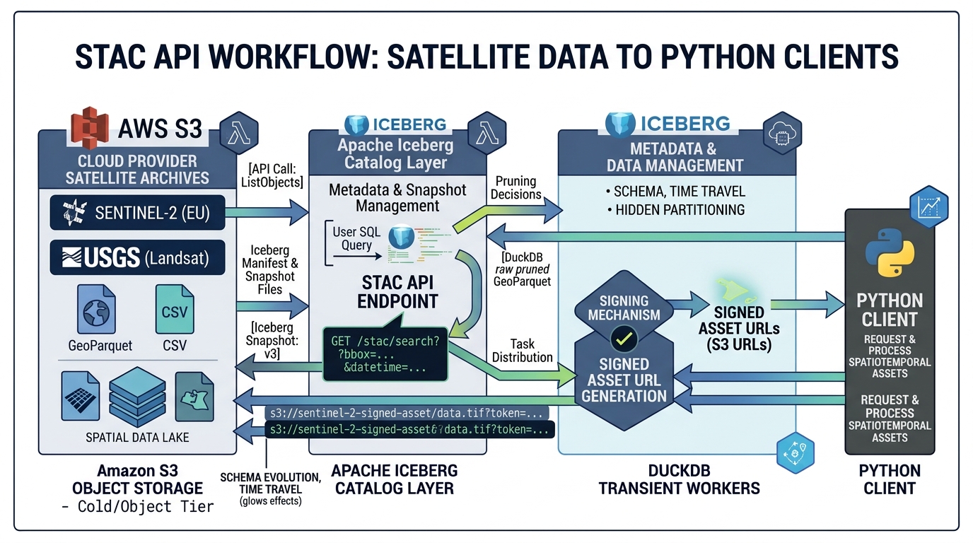
STAC (SpatioTemporal Asset Catalog) API Specification: Automating Satellite Data Pipelines

Introduction

Building Vector Tile Servers with Martin PostGIS allows modern web mapping applications to render millions of spatial records smoothly without client-side performance bottlenecks.Global satellite archives are distributed across multiple data providers, storage systems, and access interfaces. Sentinel imagery is available through Copernicus services and cloud-hosted catalogs; Landsat data is distributed through USGS and cloud platforms; and commercial providers such as Planet offer imagery through their own discovery and access services. Each provider may expose different query parameters, authentication mechanisms, metadata fields, and download workflows.

This fragmentation makes automated remote-sensing pipelines unnecessarily complicated. A script that searches one provider may require substantial modification before it can retrieve equivalent imagery from another.

The STAC API Specification for satellite data pipelines addresses this problem by providing a standardized way to describe and discover spatiotemporal assets. STAC, or SpatioTemporal Asset Catalog, defines interoperable JSON structures for representing geospatial assets, while STAC API defines HTTP interfaces for searching catalog items using geographic, temporal, and other supported filters. The specification is extensible, so providers can expose specialized metadata without abandoning the common framework.

With Python and pystac-client, engineers can automate satellite imagery discovery, select scenes with acceptable cloud-cover metadata, retrieve asset URLs, and pass cloud-optimized raster files directly into analysis pipelines.

This tutorial builds a practical workflow using Sentinel-2 Level-2A data, a public STAC endpoint, spatial and temporal filtering, signed asset URLs, and batch-processing patterns. The same architecture can be adapted to Landsat, other open satellite archives, and compatible commercial catalogs.

1. Core STAC Concepts

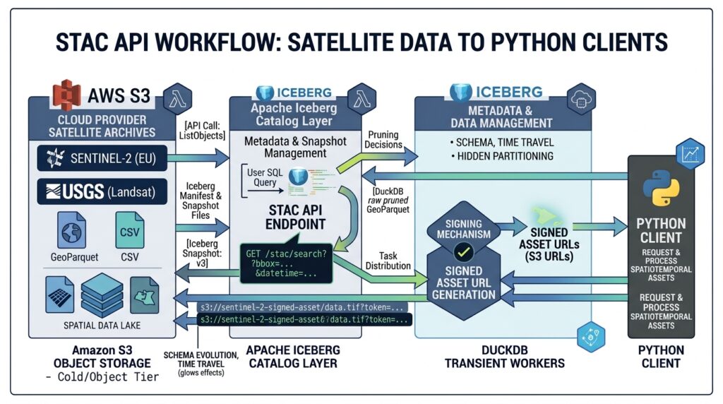
Before implementing the pipeline, it is important to understand the objects that connect a search request to the actual raster data.

1.1 Collections

A Collection groups items representing a dataset or product family. Its metadata can describe the provider, spatial and temporal extent, license, measurement characteristics, and available assets.

For example, a Sentinel-2 Level-2A collection groups observations processed to provide surface-reflectance products. The collection identifier depends on the catalog: sentinel-2-l2a is used by services such as the Microsoft Planetary Computer and Copernicus Data Space, while Earth Search’s collection identifiers depend on the API version and dataset.

Always inspect the target API’s available collections before hardcoding identifiers in production code.

1.2 Items

A STAC Item represents one cataloged observation or discrete spatiotemporal asset grouping. It is based on GeoJSON Feature structure and contains an identifier, geometry, temporal properties, links, and asset metadata.

For a Sentinel-2 scene, an Item typically describes a particular observation footprint and acquisition time. Its properties might include:

{
  "id": "example-sentinel-scene",
  "collection": "sentinel-2-l2a",
  "properties": {
    "datetime": "2025-01-15T08:12:31Z",
    "eo:cloud_cover": 7.4
  }
}

This is an illustrative fragment, not a live catalog result. Actual identifiers and metadata depend on the selected provider.

1.3 Assets

An Asset points to a resource associated with an Item. For satellite imagery, assets may represent individual spectral bands, a visual rendering, a cloud mask, scene metadata, or a thumbnail.

Common Sentinel-2 band identifiers include B02 (blue), B03 (green), B04 (red), and B08 (near-infrared). Asset names are provider-dependent, so a pipeline must inspect each Item’s asset dictionary instead of assuming every catalog uses identical keys.

Assets may be directly accessible, require temporary signed URLs, or require provider-specific authentication.

1.4 Spatiotemporal search parameters

STAC API Item Search commonly supports:

• bbox: a bounding box in longitude-latitude order, expressed as [west, south, east, north] for a two-dimensional search.

• intersects: a GeoJSON geometry for a more precise area-of-interest search.

• datetime: an acquisition time or interval using RFC 3339-compatible time expressions.

• collections: one or more collection identifiers.

• query or filter: additional property filters where the relevant API extension is supported.

The official Item Search specification defines the core parameters and paging behavior. Not every catalog supports every filtering extension, so discover the endpoint’s capabilities before relying on advanced predicates.

The typical workflow is therefore:

Define area and dates → Search Items → Filter candidate observations → Select Assets → Process or download raster data.

2. Step One: Install Python Dependencies and Connect to a STAC API

Install pystac-client, a Python library for searching STAC APIs. For this tutorial, the Microsoft Planetary Computer endpoint is used because its documentation demonstrates automatic signing of protected asset links.

python -m pip install pystac-client planetary-computer requests rasterio

The Planetary Computer STAC API is publicly discoverable, but certain asset links require signing to access the actual data. pystac-client supports a modifier callback, allowing returned STAC objects to be modified automatically.

Create a Python file named stac_satellite_pipeline.py:

from pystac_client import Clientimport planetary_computerSTAC_URL = (    "https://planetarycomputer.microsoft.com/api/stac/v1")catalog = Client.open(    STAC_URL,    modifier=planetary_computer.sign_inplace,)print("Connected to STAC API")print("Catalog title:", catalog.title)

The Client.open() method reads the catalog’s landing page and follows its advertised links. This is preferable to assuming that every provider uses identical search URLs or implements the same optional API extensions.

The modifier signs eligible asset URLs in returned objects. You do not need to manually append a token to every raster URL.

For a different service, replace the endpoint and authentication configuration with that provider’s documented access method. An API may expose public metadata while requiring authenticated access to imagery, or it may return directly accessible assets.

3. Step Two: Build Spatial and Temporal Queries

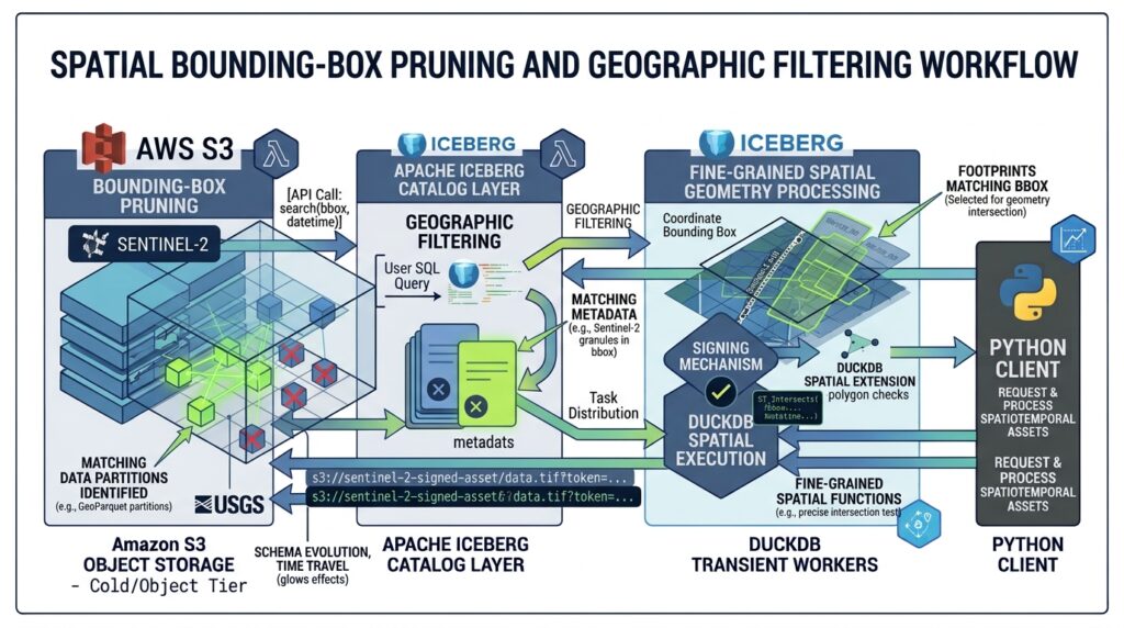
A useful satellite query narrows the search before any imagery is downloaded. This reduces unnecessary metadata processing and prevents the pipeline from retrieving scenes that are irrelevant to the study area or observation period.

For this example, the area of interest is a bounding box around Nairobi, Kenya. The time interval is January 2025, and the desired scenes have reported cloud cover below 10%.

3.1 Define the search filters

BBOX = [    36.6, -1.5,   # western and southern bounds    37.2, -1.0,   # eastern and northern bounds]DATE_RANGE = "2025-01-01/2025-02-01"MAX_CLOUD_COVER = 10search = catalog.search(    collections=["sentinel-2-l2a"],    bbox=BBOX,    datetime=DATE_RANGE,    query={        "eo:cloud_cover": {            "lt": MAX_CLOUD_COVER        }    },    max_items=100,)items = list(search.items())print(f"Matching satellite Items: {len(items)}")

The bbox values represent longitude and latitude, not latitude and longitude. The date range selects observations within the specified interval, and max_items limits how many matching Items are retrieved by the client.

The query parameter expresses a constraint on the eo:cloud_cover property. It works when the chosen catalog supports the relevant Query extension and property. If a provider rejects the query or does not advertise support for it, use its documented filtering capabilities or retrieve a bounded candidate set and apply the cloud-cover filter locally.

3.2 Sort and inspect results

Search results may contain observations with different acquisition times, cloud-cover values, and asset availability. Sort the candidates by reported cloud cover to prioritize lower-cloud scenes.

items.sort(    key=lambda item: item.properties.get(        "eo:cloud_cover", 100    ))for item in items[:10]:    cloud_cover = item.properties.get("eo:cloud_cover")    print(        item.id,        item.datetime,        f"cloud cover: {cloud_cover}%"    )

Some Items may lack a cloud-cover property. The fallback value of 100 places them at the end of the list rather than treating missing metadata as a cloud-free observation.

Important: eo:cloud_cover generally represents scene-level cloud-cover metadata, not a guarantee that the area of interest itself is cloud-free. A mostly clear scene can still contain clouds over Nairobi or another target location. For reliable analysis, apply the sensor’s cloud or scene-classification mask after obtaining the raster data.

3.3 Use intersects for irregular study areas

A bounding box is efficient for an initial search but may include large regions outside a study boundary. For an irregular watershed, agricultural district, or protected area, use a GeoJSON polygon where supported:

AOI = {    "type": "Polygon",    "coordinates": [[        [36.75, -1.35],        [37.05, -1.35],        [37.05, -1.10],        [36.75, -1.10],        [36.75, -1.35],    ]],}search = catalog.search(    collections=["sentinel-2-l2a"],    intersects=AOI,    datetime="2025-01-01/2025-02-01",    max_items=100,)

The polygon is illustrative; replace it with a validated study-area boundary. The search selects Items whose footprints intersect the requested geometry, but it does not automatically crop the rasters to the polygon.

For API compatibility, inspect the catalog’s advertised conformance classes and collection metadata. If a server does not support intersects, use bbox as an initial filter and perform precise footprint checks locally.

4. Step Three: Extract Asset Links and Handle Signing

Once Items have been discovered, the next stage is to identify the specific bands required for processing.

A four-band vegetation-analysis workflow might use blue, green, red, and near-infrared assets. Before requesting them, inspect the actual asset keys returned by the catalog.

if not items:    raise RuntimeError(        "No matching scenes found. "        "Review the area, dates, and cloud-cover threshold."    )item = items[0]print("Selected Item:", item.id)print("Acquired:", item.datetime)for key, asset in item.assets.items():    print(        key,        asset.media_type,        asset.roles,    )

This inspection is essential because collection schemas vary. One provider might expose B04 and B08, while another could use different names or represent multiple bands in a single multiband asset.

4.1 Retrieve the required band URLs

After confirming the selected Item contains the required bands, extract their asset URLs:

required_bands = ["B04", "B08"]missing_bands = [    band for band in required_bands    if band not in item.assets]if missing_bands:    raise KeyError(        f"Missing required assets: {missing_bands}"    )band_urls = {    band: item.assets[band].href    for band in required_bands}print("Available bands:", list(band_urls))

Because the catalog was opened with planetary_computer.sign_inplace, eligible asset links returned through the client are signed automatically. The URLs can therefore be passed to compatible tools without a separate manual signing step.

For individual Items retrieved through a different code path, use that provider’s documented signing process before attempting to read protected assets.

4.2 Understand signed URL lifetimes

A signed URL commonly contains a time-limited access token or signature. It is a temporary access mechanism, not a permanent asset identifier.

This creates several implications for automation:

• Re-sign asset URLs when a later job needs to access them.

• Do not assume that a URL copied from a previous run will remain valid indefinitely.

• Avoid writing tokens or complete signed URLs to public logs, repositories, or persistent manifests.

• Keep credentials in a managed secret store or workload identity rather than hardcoding them into scripts.

For reproducibility, save the collection ID, Item ID, acquisition timestamp, selected asset keys, and processing parameters. Resolve or sign the asset URLs when the processing job runs.

4.3 Generate a durable discovery manifest

A manifest separates catalog discovery from later processing. The following example stores stable metadata and the asset keys, rather than persisting potentially expiring signed URLs.

import jsonmanifest = []for item in items:    manifest.append({        "collection": item.collection_id,        "item_id": item.id,        "datetime": (            item.datetime.isoformat()            if item.datetime else None        ),        "cloud_cover": item.properties.get(            "eo:cloud_cover"        ),        "asset_keys": [            key for key in ("B04", "B08")            if key in item.assets        ],    })with open("satellite_manifest.json", "w") as f:    json.dump(manifest, f, indent=2)print(f"Saved {len(manifest)} records")

This manifest is a durable record of discovery. A later processing worker can retrieve the recorded Items, refresh their signed asset links, and execute the required raster operations.

5. Step Four: Automate Downloads or Process Imagery in Place

The main advantage of STAC is that it separates discovery from data access. Once an Item and its assets have been identified, the pipeline can either download the required rasters or pass their URLs directly to a cloud-capable processing library.

The right approach depends on the asset format, network environment, and processing requirements.

5.1 Download selected assets in batches

For workflows that require local copies, stream the requested assets to disk. Streaming avoids loading the entire raster into memory.

from pathlib import Pathimport requestsoutput_dir = Path("satellite_data")output_dir.mkdir(parents=True, exist_ok=True)def download_asset(url, destination):    with requests.get(        url,        stream=True,        timeout=(15, 180),    ) as response:        response.raise_for_status()        with open(destination, "wb") as output:            for chunk in response.iter_content(                chunk_size=1024 * 1024            ):                if chunk:                    output.write(chunk)for band, url in band_urls.items():    destination = output_dir / (        f"{item.id}_{band}.tif"    )    download_asset(url, destination)    print(f"Downloaded {band}: {destination}")

This is a minimal download function, not a complete production transfer manager. A production implementation should add bounded retries with exponential backoff for transient network failures, temporary-file handling, integrity checks, and idempotent output naming. For very large assets, avoid restarting an entire download unnecessarily when the server supports valid HTTP range requests.

The script also assumes each selected asset is a GeoTIFF. Inspect the asset’s media type and file format before choosing an output extension or raster reader.

5.2 Process cloud-hosted rasters without downloading the full file

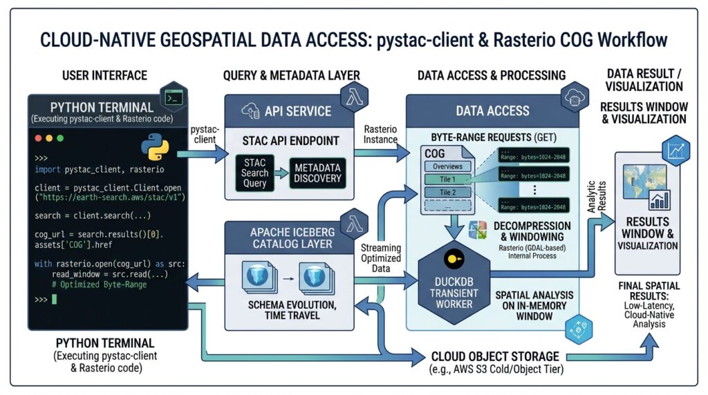
Where assets are cloud-optimized GeoTIFFs (COGs), a compatible GDAL-backed reader can often retrieve only the byte ranges required for the requested windows. For deeper raster transformation techniques, you can also explore our guide on Optimizing Enterprise Web Maps with Cloud-Optimized GeoTIFF (COG) Architecture. This is particularly useful when the study area occupies a small portion of a large satellite scene.

For example, Rasterio can open a signed URL directly when the underlying GDAL installation supports remote HTTP access and the source allows the required range requests:

import rasteriourl = band_urls["B04"]with rasterio.open(url) as src:    print("CRS:", src.crs)    print("Raster dimensions:", src.width, src.height)    print("Bounds:", src.bounds)

Opening the file does not necessarily download the full raster. Reading a complete band into memory, however, may transfer substantial data. Use appropriate windows or a geometry-based crop when only part of a scene is needed, and transform the study-area geometry into the raster’s CRS before calculating the pixel window.

The asset’s signed URL must still be valid when GDAL accesses it. If the source cannot be read directly from your environment, use the provider’s supported download or authentication workflow instead.

6. Build an Automated Satellite Ingestion Pipeline

The preceding components can be assembled into a repeatable remote-sensing job:

For an operational implementation, the pipeline should be idempotent: rerunning the same request must not create duplicate output products or overwrite valid results unexpectedly. Use the collection ID, Item ID, asset selection, and processing version to create reproducible job keys.

Pagination also matters. STAC APIs may return results in multiple pages, and pystac-client handles the advertised next links when iterating search results. Set a deliberate result limit and process items incrementally rather than assuming that one API response contains every matching scene.

For larger workloads, separate discovery and raster execution into different jobs. One process can write the durable discovery manifest; multiple workers can then process individual Items or spatial tiles in parallel. This avoids coupling catalog availability to the runtime of lengthy raster operations.

6.1 Operational safeguards

Before publishing results, check that each Item meets the requirements of the analysis. A low cloud percentage does not replace pixel-level cloud masking. Confirm the expected CRS, spatial resolution, band availability, radiometric scale, and data-quality flags.

Use bounded concurrency to avoid overwhelming a public catalog or creating excessive download traffic. Apply retry policies to temporary network errors, but fail clearly on permanent authorization errors, missing assets, or unsupported formats.

Finally, record the Item IDs and acquisition times used by each run. These identifiers make it easier to reproduce an output or investigate changes when providers update catalog contents or asset access policies.

7. SEO Interlinking and Further Reading

STAC discovery is most powerful when connected to downstream raster analysis and publication workflows. Recommended internal links include:

• Google Earth Engine Change Detection Tutorial — for using time-series imagery to detect land-cover and environmental change.

• Building a Cloud-Optimized GeoTIFF (COG) Web Map Architecture — for serving raster products efficiently over HTTP.

• Optimizing Raster Processing Performance with GDAL Multi-Threading and VRT Files — for improving raster transformation and processing performance.

Use these as internal links after confirming that the corresponding articles exist at those URLs.

Image placeholder

[Image 1: Python terminal showing STAC API query execution and returned matching satellite scene items]

Alt text: “Terminal screenshot showing Python code executing a STAC API query to discover cloud-filtered Sentinel-2 satellite imagery assets.”

For authoritative implementation details, consult the official STAC Specification, the STAC API Item Search specification, and the pystac-client documentation. For Copernicus Sentinel imagery, the Copernicus Data Space STAC documentation describes available collections and supported query extensions.

Conclusion

The STAC API Specification provides a consistent foundation for automating satellite data discovery across diverse geospatial catalogs. By combining pystac-client with spatial and temporal filtering, cloud-cover metadata, asset inspection, and provider-specific signing, remote-sensing engineers can build reproducible pipelines that identify suitable imagery without manually browsing individual scenes.

The essential architectural principle is to separate discovery, access, and processing. STAC identifies the right observations, signed or public asset URLs provide access, and tools such as Rasterio and GDAL perform the raster analysis. With pagination, validation, retry logic, and durable manifests, this workflow can evolve from a simple Python script into a scalable satellite data ingestion service.