
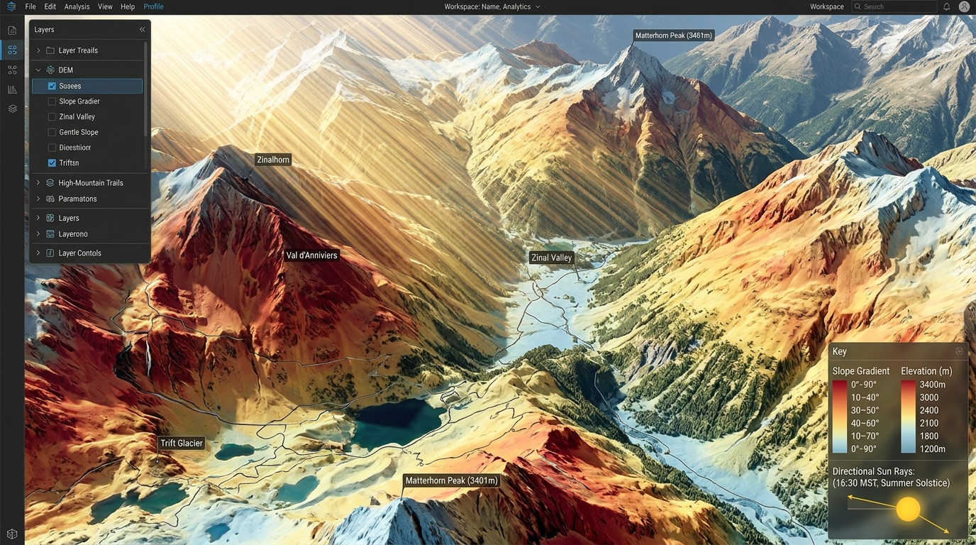
3D Solar Radiation Modeling on Complex Terrain Using DEMs and GRASS GIS
Utility-scale solar photovoltaic (PV) deployment has expanded from flat, arid plains into complex, mountainous topographies. Estimating solar yield across rugged landscapes presents significant spatial modeling challenges: standard planar insolation models fail to account for microclimatic fluctuations, terrain-induced self-shadowing, elevated horizon obstructions, and anisotropic diffuse sky radiation. Evaluating renewable energy potential across alpine valleys or steep hillsides requires 3D solar radiation modeling grounded in high-resolution Digital Elevation Models (DEMs).
GRASS GIS remains an open-source standard for physical geographic processing. Its flagship solar modeling module,
r.sun, implements precise clear-sky and real-sky radiation algorithms based on the European Solar Radiation Atlas (ESRA) formulation. By parameterizing atmospheric attenuation, elevation gradients, ground albedo, and dynamic ray-traced shadow rasters, GIS analysts can simulate direct beam, diffuse, and ground-reflected radiation flux ($W/m^2$ or $Wh/m^2$) across multi-temporal schedules.This technical guide provides a step-by-step workflow for configuring, executing, and analyzing 3D solar radiation models using DEMs within GRASS GIS.
Technical Foundations: Solar Radiation Mechanics in Complex Topography
Accurate solar site selection across non-planar landscapes depends on modeling three primary solar radiation components:
-
Direct Normal & Beam Irradiance ($I_{beam}$): Solar energy arriving in a straight vector from the solar disk. Topographic slope ($\gamma$) and aspect ($\alpha$) determine the local incidence angle ($\theta$). Shadowing from adjacent ridge-lines cuts off direct beam transmission during low sun angles.
-
Diffuse Sky Irradiance ($I_{diffuse}$): Scrambled photon flux scattered by atmospheric particles, aerosols, and cloud cover. In complex terrain, surrounding topography blocks portions of the sky dome, requiring calculation of the local Sky View Factor (SVF).
-
Ground-Reflected Radiation ($I_{reflected}$): Secondary flux bounced onto a surface from surrounding terrain, governed by ground surface albedo ($\rho$). Highly reflective surfaces like snow-covered slopes significantly boost total incident radiation.
The total global solar radiation ($I_{global}$) incident on a sloped surface is expressed as:
$$I_{global} = I_{beam} \cdot \cos(\theta) + I_{diffuse} + I_{reflected}$$
                Sun Vector
                  \
                   \
    +---------------V---------------+
    |       Direct Beam (I_beam)    |
    +-------------------------------+
                   |
     +-------------+-------------+
     |                           |
     V                           V
+-------------------+   +-------------------+
| Shadow Ray-Tracing|   | Atmospheric Scattering|
| (r.horizon maps)  |   | (Linke Turbidity) |
+-------------------+   +-------------------+
     |                           |
     +-------------+-------------+
                   |
                   V
     +---------------------------+
     | Diffuse Irradiance (SVF)  |
     +---------------------------+
                   |
                   V
     +---------------------------+
     | Ground-Reflected (Albedo) |
     +---------------------------+
                   |
                   V
     +---------------------------+
     |   Total Global Solar yield|
     |        (r.sun output)     |
     +---------------------------+
Without accounting for terrain occlusions and surface orientation, static 2D planar models systematically overestimate annual energy yields in mountain valleys by up to 35%.
Workflow Implementation (GRASS GIS)
Step 1: Preparing High-Resolution DEMs & Horizon Obstacle Inputs
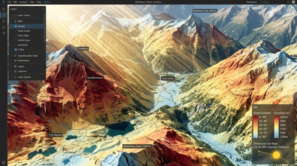
Precise solar flux modeling requires derived topographic layers: slope, aspect, and horizon elevation angles. High-density terrain datasets (such as USGS 3DEP or LiDAR canopy height model extraction) serve as foundational rasters.
First, set the computational region matching your high-resolution DEM, and calculate slope and aspect layers:
Bash
# Set computational region to match DEM resolution and extent
g.region raster=dem_1m -p

# Generate Slope and Aspect rasters (r.slope.aspect expects degrees)
r.slope.aspect elevation=dem_1m \
    slope=slope_deg \
    aspect=aspect_deg \
    format=degrees \
    precision=FCELL
Computing Horizon Occlusion Files (r.horizon)
Terrain shadowing is calculated by determining the horizon height—the maximum vertical elevation angle of blocking terrain—along discrete azimuthal step angles around every cell.
Bash
# Compute horizon raster maps every 30 degrees (12 directional rasters)
r.horizon elevation=dem_1m \
    step=30 \
    bufferzone=5000 \
    output=horizon_angle \
    maxdistance=10000
Performance Optimization Note: Generating horizon maps across large spatial extents is computationally intensive. Pre-processing rasters using GDAL multi-threading raster optimization techniques before importing them into your GRASS database will speed up tile execution times.
Step 2: Configuring Atmospheric Parameters & Surface Attributes
r.sun requires atmospheric attenuation coefficients and surface reflectance indices:-
Linke Turbidity Factor ($T_L$): Quantifies clear-sky atmospheric attenuation caused by water vapor and aerosols. Typical values range from $T_L = 2.0$ (clean, high-altitude alpine air) to $T_L = 5.0+$ (polluted or humid lowlands).
-
Ground Albedo ($\rho$): Dimensionless reflection coefficient ranging from $0.15–0.25$ for typical vegetated terrain, up to $0.80–0.90$ for snow-covered peaks.
-
Elevation Map: Accounts for atmospheric barometric pressure reductions over high-altitude terrain, decreasing Rayleigh scattering losses.
Create uniform or spatially explicit rasters for Linke turbidity and albedo:
Bash
# Create a spatial Linke Turbidity map (e.g., constant 2.5 for alpine region)
r.mapcalc expression="linke_turb = 2.5"

# Create Ground Albedo raster (e.g., 0.20 baseline, elevated for snow zones)
r.mapcalc expression="albedo_grid = if(dem_1m > 2500, 0.65, 0.20)"
Step 3: Executing r.sun for Multi-Temporal Irradiance Grids
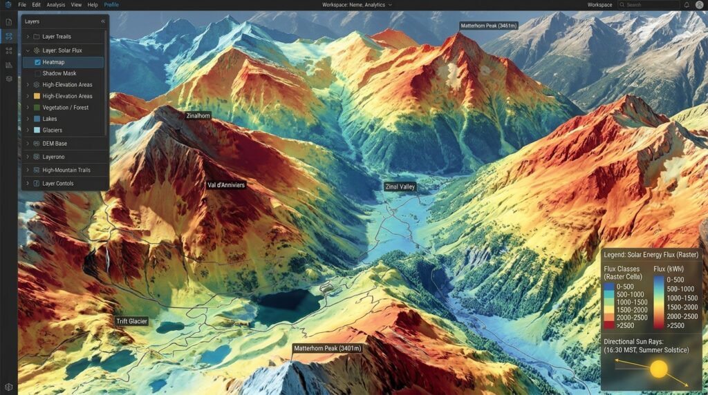
The
r.sun module runs in two primary operational modes:-
Mode 1 (Instantaneous Mode): Calculates solar irradiance ($W/m^2$) at a specific minute/hour.
-
Mode 2 (Integrated Mode): Computes cumulative daily solar radiation ($Wh/m^2 \cdot \text{day}$) for a specified day-of-year (
day=1..365).
Executing Mode 2 for Solstice Solar Yields (Day 172 – Summer Solstice)
Bash
# Compute integrated daily irradiance for Day 172 (June 21) using pre-calculated horizon rasters
r.sun elevation=dem_1m \
    aspect=aspect_deg \
    slope=slope_deg \
    linke=linke_turb \
    albedo=albedo_grid \
    horizon_step=30 \
    horizon_basename=horizon_angle \
    day=172 \
    step=0.5 \
    beam_rad=beam_day172 \
    diff_rad=diff_day172 \
    refl_rad=refl_day172 \
    glob_rad=global_day172
Automated Scripting for Annual Cumulative Yields
To calculate total annual energy yield ($kWh/m^2 \cdot \text{year}$), loop
r.sun across representative monthly sampling intervals or every day of the calendar year (365 iterations):Python
#!/usr/bin/env python3
import grass.script as gscript

# Loop through representative days of each month
sample_days = [17, 47, 75, 105, 135, 162, 198, 228, 258, 288, 318, 344]
days_in_month = [31, 28, 31, 30, 31, 30, 31, 31, 30, 31, 30, 31]

monthly_rasters = []

for day, weight in zip(sample_days, days_in_month):
    beam_out = f"beam_day_{day}"
    diff_out = f"diff_day_{day}"
    glob_out = f"glob_day_{day}"

    print(f"Executing r.sun for Day-of-Year: {day}")
    gscript.run_command(
        'r.sun',
        elevation='dem_1m',
        aspect='aspect_deg',
        slope='slope_deg',
        linke='linke_turb',
        albedo='albedo_grid',
        horizon_step=30,
        horizon_basename='horizon_angle',
        day=day,
        step=1.0,
        beam_rad=beam_out,
        diff_rad=diff_out,
        glob_rad=glob_out,
        overwrite=True
    )

    # Scale daily yield Wh/m2 to monthly kWh/m2
    month_calc = f"month_kWh_{day} = ({glob_out} * {weight}) / 1000.0"
    gscript.mapcalc(month_calc)
    monthly_rasters.append(f"month_kWh_{day}")

# Sum all monthly layers into annual total radiation map (kWh/m2/year)
annual_expression = f"annual_solar_yield_kWh = {' + '.join(monthly_rasters)}"
gscript.mapcalc(annual_expression)
print("Annual Solar Radiation Yield Computed Successfully.")
Step 4: Extracting Zonal Statistics for Optimal Site Selection
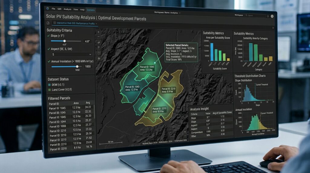
Raw annual irradiance grids must be filtered through spatial engineering constraints to pinpoint suitable utility-scale PV deployment zones. High potential sites typically require:
-
Annual Insolation: $> 1,650 \text{ kWh/m}^2/\text{year}$
-
Terrain Slope: $< 10^\circ$ (minimizes civil earthwork costs)
-
Aspect Orientation: $135^\circ \text{ to } 225^\circ$ (South-facing in Northern Hemisphere)
-
Proximity to Infrastructure: Avoiding severe valley shading zones while remaining near transmission corridors.
Bash
# Filter prospective development zones meeting technical thresholds
r.mapcalc expression="candidate_pv_sites = if(annual_solar_yield_kWh >= 1650 && slope_deg <= 10.0 && aspect_deg >= 135 && aspect_deg <= 225, 1, null())"

# Vectorize candidate patches into discrete polygonal zones
r.to.vect input=candidate_pv_sites output=pv_candidate_parcels type=area

# Extract zonal radiation yield statistics per polygon parcel
v.rast.stats map=pv_candidate_parcels \
    raster=annual_solar_yield_kWh \
    column_prefix=sol \
    method=average,stddev,maximum
By querying the resultant attribute table (
sol_average), site selection teams can quantitatively rank candidate land parcels based on projected megawatt-hour (MWh) generation yields per unit area. Similar spatial modeling workflows can also be adapted to granular urban environments, such as urban rooftop solar analysis.
Technical Summary & Renewable Energy Takeaways
3D solar radiation modeling with
r.sun in GRASS GIS allows developers to evaluate topography-driven solar potential with fine-grained accuracy.Key Modeling Takeaways:
-
Accounting for Horizon Occlusion: Using
r.horizonto model self-shadowing terrain prevents overestimating energy yields in mountainous areas. -
Spectral Sensitivity Matters: Tuning atmospheric turbidity ($T_L$) and albedo inputs allows models to account for high-altitude air clarity and ground reflections from snow cover.
-
Multi-Temporal Integration: Combining daily irradiance runs into weighted annual layers provides reliable inputs for financial models, site selection, and utility capacity planning.
Deploying scriptable, open-source GIS pipelines ensures that solar capacity models remain transparent, reproducible, and scalable across complex terrain anywhere in the world.