
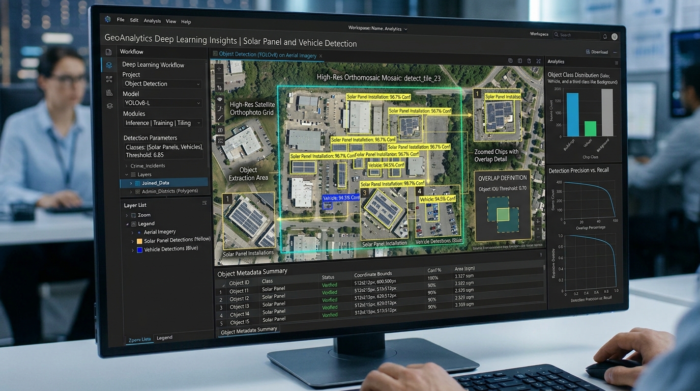
Fine-Tuning YOLOv8 for Automated Object Detection on High-Resolution Satellite Orthophotos
Introduction
In the fields of Geographic Information Systems (GIS) and remote sensing, extracting features from high-resolution aerial and satellite imagery has traditionally relied on pixel-based classification, spectral indices (such as NDVI or NDBI), and classic morphological image processing. While these methods are computationally lightweight, they frequently struggle with spatial context, scale variations, and complex urban backgrounds.
Modern deep learning-based object detection—specifically Ultralytics YOLOv8—has revolutionized automated feature extraction. By treating geospatial object detection as an end-to-end regression and classification problem, YOLOv8 enables real-time, high-precision identification and counting of infrastructure elements like vehicles, solar panels, buildings, and wind turbines across vast regional orthomosaics.
Preparing Training Data
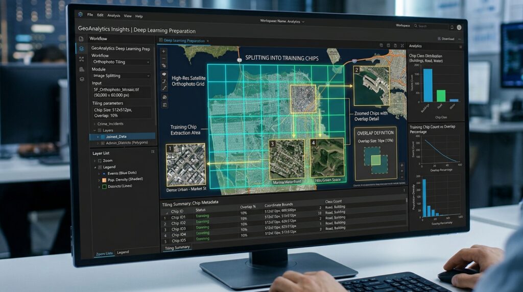
High-resolution GeoTIFF orthophotos often span gigabytes or terabytes, rendering them too large to pass directly into convolutional neural networks. Preparing training data requires systematic tiling and spatial reference management.
Tiling High-Resolution GeoTIFF Orthophotos
Deep learning models typically operate on fixed input dimensions, such as $640 \times 640$ pixels. Using Python libraries like
rasterio and gdal, large GeoTIFF orthophotos must be systematically sliced into smaller chips. To prevent edge-artifact clipping where objects are cut off mid-feature, it is standard practice to incorporate an overlap buffer (e.g., 10% to 15%) between adjacent tiles.Python
import rasterio
from rasterio.windows import Window
import os

def tile_geotiff(image_path, output_dir, tile_size=640, overlap=64):
    os.makedirs(output_dir, exist_ok=True)
    with rasterio.open(image_path) as src:
        width = src.width
        height = src.height

        stride = tile_size - overlap
        for y in range(0, height, stride):
            for x in range(0, width, stride):
                w = min(tile_size, width - x)
                h = min(tile_size, height - y)

                window = Window(x, y, w, h)
                transform = rasterio.windows.transform(window, src.transform)

                kwargs = src.meta.copy()
                kwargs.update({
                    'height': h,
                    'width': w,
                    'transform': transform
                })

                out_path = os.path.join(output_dir, f"tile_{x}_{y}.tif")
                with rasterio.open(out_path, 'w', **kwargs) as dst:
                    dst.write(src.read(window=window))
Annotating Bounding Boxes and Spatial Coordinate Conversions
Annotations for YOLOv8 must be formatted as plain text files (
.txt) corresponding to each image tile, where each row represents a bounding box using normalized center coordinates:$$\text{class\_id } x_{center} y_{center} width height$$
When vector ground truth data exists as GIS shapefiles or GeoJSON layers in real-world geographic coordinate systems (e.g., EPSG:4326 WGS84 or local UTM zones), you must transform those geometries into pixel space relative to each individual tile’s affine transformation matrix before writing the YOLO text labels.
Step-by-Step Code Walkthrough
1. Setting up the Environment and Dataset Configuration YAML
First, install the Ultralytics package and initialize your dataset configuration file (
dataset.yaml), which points to your training and validation image directories and defines your target classes.YAML
# dataset.yaml
path: /path/to/geospatial_dataset
train: images/train
val: images/val

names:
  0: solar_panel
  1: vehicle
  2: building_footprint
2. Fine-Tuning YOLOv8: Training a Pre-Trained Model
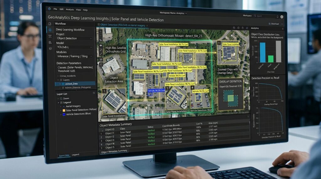
Load a pre-trained YOLOv8 weights file (e.g.,
yolov8x.pt) and fine-tune the model on your custom aerial dataset. Fine-tuning leverages transfer learning, allowing the network to adapt its feature extractors to overhead remote sensing perspectives.Python
from ultralytics import YOLO

# Load a pre-trained YOLOv8 model (e.g., Extra Large model for high accuracy)
model = YOLO("yolov8x.pt")

# Fine-tune the model on custom geospatial classes
results = model.train(
    data="dataset.yaml",
    epochs=50,
    imgsz=640,
    batch=16,
    device=0,
    workers=8,
    box=7.5,
    cls=0.5,
    patience=10,
    save=True,
    project="geospatial_yolo",
    name="solar_panel_detector"
)
3. Running Batch Inference on Large Mosaic Orthophotos
Once trained, the model can perform batch inference across extensive regional orthomosaics. To learn more about efficient raster processing workflows prior to inference, check out our guide on Python raster processing techniques.
Python
import glob

# Load the fine-tuned custom weights
trained_model = YOLO("geospatial_yolo/solar_panel_detector/weights/best.pt")

# Run batch prediction across all inference tiles
inference_results = trained_model.predict(
    source="/path/to/inference_tiles/*.tif",
    conf=0.45,
    iou=0.5,
    save_txt=True,
    save_conf=True
)
4. Converting Pixel-Space Predictions to Geographic Vector Coordinates
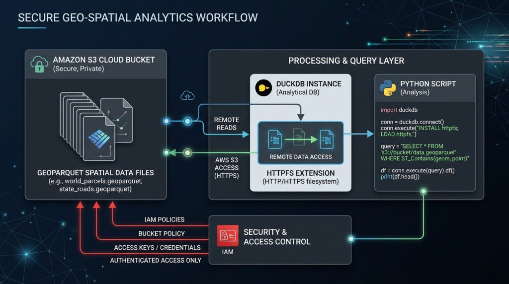
YOLOv8 outputs predictions in pixel coordinates relative to each image tile. To integrate these detections into GIS software for spatial analysis, you must convert them back into real-world geographic coordinates using
rasterio and geopandas.Python
import geopandas as gpd
from shapely.geometry import box
import rasterio

def pixels_to_gis(tile_tif_path, yolo_txt_path, output_shp_path):
    with rasterio.open(tile_tif_path) as src:
        transform = src.transform
        crs = src.crs

        geometries = []
        confidences = []

        with open(yolo_txt_path, 'r') as f:
            for line in f.readlines():
                parts = line.strip().split()
                cls_id, x_c, y_c, w, h, conf = map(float, parts)

                img_w, img_h = src.width, src.height
                x_min = (x_c - w / 2) * img_w
                x_max = (x_c + w / 2) * img_w
                y_min = (y_c - h / 2) * img_h
                y_max = (y_c + h / 2) * img_h

                # Convert pixel coordinates to spatial coordinates using affine transform
                ul_x, ul_y = rasterio.transform.xy(transform, y_min, x_min)
                lr_x, lr_y = rasterio.transform.xy(transform, y_max, x_max)

                geom = box(ul_x, lr_y, lr_x, ul_y)
                geometries.append(geom)
                confidences.append(conf)

        gdf = gpd.GeoDataFrame({'confidence': confidences, 'geometry': geometries}, crs=crs)
        gdf.to_file(output_shp_path, driver='ESRI Shapefile')
For more advanced vector post-processing workflows—such as refining building polygons derived from bounding boxes—refer to our tutorial on Segment Anything Model (SAM) building extraction in QGIS.
Conclusion
Fine-tuning Ultralytics YOLOv8 for high-resolution satellite orthophotos bridges the gap between modern computer vision and traditional geospatial analytics. By combining systematic raster tiling, transfer learning, and affine transformation pipelines, developers and geospatial scientists can automate large-scale feature extraction with exceptional speed and accuracy.b