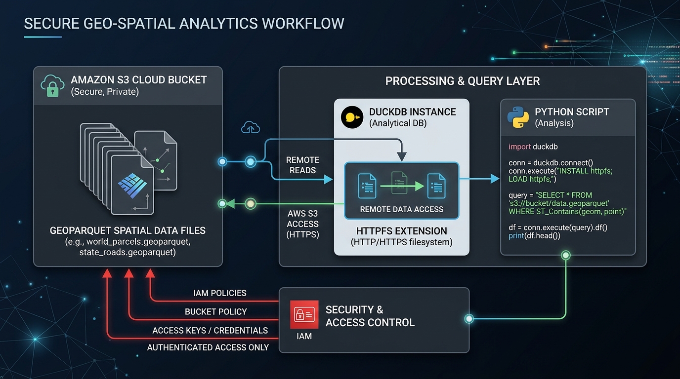
Querying GeoParquet Files Directly from Amazon S3 Using DuckDB and Python

Introduction: Building a Serverless Spatial Data Lake

If you want to efficiently Query GeoParquet DuckDB Amazon S3 Python workflows, cloud-native spatial engineering makes it possible to analyze large vector datasets without traditional database servers. Geospatial data engineering increasingly relies on cloud object storage rather than traditional database servers. Large vector datasets—road networks, administrative boundaries, building footprints, and environmental observations—can be stored as Parquet files in Amazon S3 and queried when needed.

Parquet is a columnar storage format that supports compression, column projection, and metadata-based filtering. GeoParquet extends this format with geospatial metadata, including geometry encoding and coordinate reference system information. Together, they provide a foundation for cloud-native vector analytics.

DuckDB brings an analytical SQL engine directly into Python. With its httpfs extension, DuckDB can read from and write to S3-compatible object storage. Its spatial extension adds functions for geometry processing, spatial joins, and coordinate transformations. This lets developers analyze large remote datasets without first downloading every file or operating a conventional database server.

In this tutorial, you will learn how to securely configure S3 access, query remote GeoParquet datasets, apply spatial filters and ST_Intersects joins, and export optimized results back to cloud storage.

The examples target DuckDB 1.5 or later. Current DuckDB versions support GeoParquet reading and writing in core, while spatial operations still require the spatial extension. See the GeoParquet distribution guidance.

1. Prerequisites and Environment Setup

You will need Python 3.10 or later, access to an Amazon S3 bucket, and permission to read the source objects. Exporting results also requires write permissions on the destination prefix.

Install the Python dependencies

Create a virtual environment and install the required packages:

python -m venv .venv

Activate it on Windows:

.venv\Scripts\Activate.ps1

Or on Linux and macOS:

source .venv/bin/activate

Install the libraries:

python -m pip install "duckdb>=1.5.0" geopandas pyarrow

DuckDB performs the main SQL processing. GeoPandas is useful for validating exported spatial data or continuing analysis in Python, while PyArrow provides additional Parquet inspection and interoperability tools.

Configure AWS credentials securely

Install and configure the AWS CLI. For local development, an AWS IAM Identity Center profile or another supported AWS credential provider is preferable to embedding access keys in Python source code.

For example, if your organization provides an SSO profile named geo-analytics:

aws configure sso --profile geo-analytics
aws sso login --profile geo-analytics

On Windows PowerShell, select the profile for the current terminal:

$env:AWS_PROFILE = "geo-analytics"

On Linux or macOS:

export AWS_PROFILE=geo-analytics

Verify the active identity:

aws sts get-caller-identity

The identity needs s3:GetObject for source files and, when querying wildcard paths, appropriate s3:ListBucket permissions. For output, it also needs the required upload permissions. If the bucket uses AWS KMS encryption, the relevant KMS permissions may be required as well.

For workloads running on AWS, an appropriately restricted IAM role is often preferable to an interactive profile.

2. Initialize DuckDB and Configure S3 Access

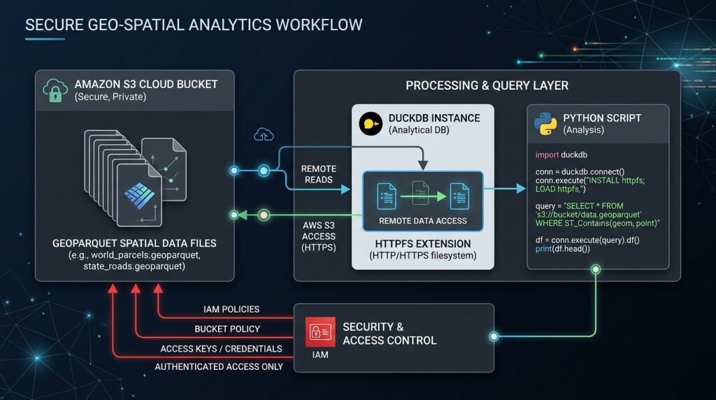
DuckDB’s httpfs extension enables remote object-storage access. The aws extension provides support for AWS credential-chain authentication, which can obtain credentials from supported providers instead of requiring keys in application code.

Create a file named query_geoparquet.py:

import duckdb

con = duckdb.connect(":memory:")

# Install extensions once; subsequent runs can use the local cache.
con.execute("INSTALL httpfs")
con.execute("INSTALL aws")
con.execute("INSTALL spatial")

# Load extensions into this connection.
con.execute("LOAD httpfs")
con.execute("LOAD aws")
con.execute("LOAD spatial")

# Use the AWS credential chain rather than hard-coded credentials.
con.execute("""
    CREATE OR REPLACE SECRET s3_data (
        TYPE s3,
        PROVIDER credential_chain,
        REGION 'eu-west-1',
        SCOPE 's3://my-geo-bucket/'
    )
""")

Replace eu-west-1 with the actual bucket region and my-geo-bucket with your bucket name. The scoped secret limits where DuckDB applies those credentials; AWS IAM policies remain responsible for enforcing the actual permissions.

This configuration uses the AWS credential chain, allowing DuckDB to work with supported credentials from the environment, profiles, SSO, or AWS roles. See the DuckDB S3 API and authentication documentation.

Security note: Do not place secret access keys in committed Python files, notebooks, or SQL scripts. Use temporary credentials or roles where possible, and grant access only to the required bucket prefixes.

3. Query GeoParquet Files Directly from S3

Assume the bucket contains a dataset organized as follows:

s3://my-geo-bucket/
└── raw/
    ├── events/
    │   ├── year=2025/
    │   │   └── part-000.parquet
    │   └── year=2026/
    │       └── part-001.parquet
    └── administrative_boundaries/
        └── boundaries.parquet

The event files contain columns such as event_id, event_date, event_type, and geom. The geometry column stores spatial features in GeoParquet format.

Run a basic remote query

After configuring the connection, query the dataset directly:

query = """
    SELECT
        event_type,
        COUNT(*) AS event_count
    FROM read_parquet(
        's3://my-geo-bucket/raw/events/**/*.parquet',
        hive_partitioning = true
    )
    WHERE event_date >= DATE '2026-01-01'
      AND event_date <  DATE '2026-02-01'
    GROUP BY event_type
    ORDER BY event_count DESC
"""

result = con.execute(query).fetchdf()
print(result)

The wildcard reads matching Parquet files, and hive_partitioning = true enables inference of partition values from directory names such as year=2026.

The exact directory layout and date column must match your source dataset. If the year is encoded only in the path and there is no event_date column, filter on the inferred year partition column instead.

DuckDB reads the Parquet metadata and requests the data required by the query from S3. It does not require a complete local download of every source file. However, a broad query that reads most columns and rows can still transfer a substantial amount of data.

Reduce unnecessary I/O

Use column projection and selective predicates. For example:

SELECT event_id, event_type, geom
FROM read_parquet(
    's3://my-geo-bucket/raw/events/**/*.parquet',
    hive_partitioning = true
)
WHERE year = 2026
  AND event_type = 'flood';

The query requests only the columns it needs. Partition pruning and Parquet row-group statistics may also eliminate some data reads when the dataset is organized appropriately and the relevant statistics are available.

For very large datasets, avoid SELECT * unless all columns are genuinely needed. Network transfer, decompression, and geometry decoding can otherwise dominate the query.

4. Apply Spatial Filters and Predicate Pushdown

Spatial analysis introduces a challenge: exact geometric operations can be expensive when applied to millions of features. A common strategy is to filter by a bounding box first, then run an exact spatial predicate on the remaining candidates.

For the following example, assume the input GeoParquet file contains a geom geometry column and an optional bbox struct with the fields xmin, ymin, xmax, and ymax. This is a common GeoParquet bounding-box layout; verify your actual schema before using the query.

Define an area of interest

The example uses a rectangular region in longitude and latitude:

aoi_wkt = """
POLYGON ((
    36.6 -1.45,
    37.1 -1.45,
    37.1 -1.05,
    36.6 -1.05,
    36.6 -1.45
))
"""

These coordinates assume the source geometries are in longitude/latitude coordinates compatible with this area. Confirm the source CRS from the GeoParquet metadata, and reproject data if necessary before comparing geometries.

Use ST_GeomFromText to create the area geometry and filter the source:

spatial_filter_query = f"""
    WITH aoi AS (
        SELECT ST_GeomFromText('{aoi_wkt}') AS geom
    )
    SELECT
        e.event_id,
        e.event_type,
        e.geom
    FROM read_parquet(
        's3://my-geo-bucket/raw/events/**/*.parquet',
        hive_partitioning = true
    ) AS e
    CROSS JOIN aoi
    WHERE e.bbox.xmax >= 36.6
      AND e.bbox.xmin <= 37.1
      AND e.bbox.ymax >= -1.45
      AND e.bbox.ymin <= -1.05
      AND ST_Intersects(e.geom, aoi.geom)
"""

events_in_area = con.execute(spatial_filter_query).fetchdf()
print(events_in_area.head())

The four bounding-box comparisons are a coarse filter: they retain geometries whose bounding boxes overlap the rectangular area. ST_Intersects then performs the exact geometry test.

If your input has no bbox struct, remove these four predicates and use ST_Intersects alone, or create a reusable dataset containing bounding boxes during preprocessing.

Important performance distinction: These bbox conditions reduce the number of exact geometric tests, but they do not automatically guarantee that S3 bytes or Parquet row groups will be skipped. Effective I/O pruning depends on file organization, row-group statistics, partitioning, and the query engine’s supported optimizations. Spatially ordered files with useful bounding-box statistics are generally more selective than randomly ordered records.

DuckDB’s spatial predicates are documented in the Spatial Functions reference.

5. Execute a Spatial Join with ST_Intersects

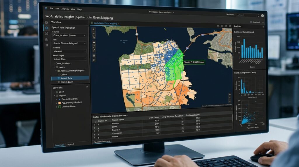
A common use case is assigning events to administrative areas. Suppose the event dataset contains point geometries while the administrative dataset contains polygon geometries. Both datasets have a geom column and a bbox struct.

The query below first limits both datasets to the same region and then joins their geometries:

spatial_join_query = """
    WITH events AS (
        SELECT event_id, event_type, geom
        FROM read_parquet(
            's3://my-geo-bucket/raw/events/**/*.parquet',
            hive_partitioning = true
        )
        WHERE bbox.xmax >= 36.6
          AND bbox.xmin <= 37.1
          AND bbox.ymax >= -1.45
          AND bbox.ymin <= -1.05
    ),
    areas AS (
        SELECT area_id, area_name, geom
        FROM read_parquet(
            's3://my-geo-bucket/raw/administrative_boundaries/*.parquet'
        )
        WHERE bbox.xmax >= 36.6
          AND bbox.xmin <= 37.1
          AND bbox.ymax >= -1.45
          AND bbox.ymin <= -1.05
    )
    SELECT
        a.area_id,
        a.area_name,
        e.event_type,
        COUNT(*) AS event_count
    FROM events AS e
    JOIN areas AS a
      ON ST_Intersects(e.geom, a.geom)
    GROUP BY
        a.area_id,
        a.area_name,
        e.event_type
    ORDER BY event_count DESC
"""

join_result = con.execute(spatial_join_query).fetchdf()
print(join_result)

The example assumes the bounding-box fields exist in both sources and the coordinates share a compatible CRS. Modify the S3 paths and field names to match your schema.

ST_Intersects is an exact spatial predicate, whereas bbox comparisons are only a preliminary overlap test. For points that lie on a polygon boundary, ST_Intersects returns true. If your business rule requires strictly interior points, investigate the appropriate predicate, such as ST_Within, and validate its boundary behavior.

For large joins, reduce each side as much as possible before joining. Partitioning by geographic area, selecting only necessary columns, spatially ordering features, and maintaining compact row groups can improve performance. Do not assume that a spatial predicate alone guarantees an optimal join plan; inspect it with DuckDB’s EXPLAIN ANALYZE.

6. Export Filtered Results Back to Amazon S3

Once analysis is complete, DuckDB can write results directly to S3 using the COPY statement. This avoids an intermediate step in which Python downloads the entire result to local storage before uploading it again.

For example, export the spatially filtered events:

export_query = """
    COPY (
        SELECT
            event_id,
            event_type,
            geom
        FROM read_parquet(
            's3://my-geo-bucket/raw/events/**/*.parquet',
            hive_partitioning = true
        )
        WHERE bbox.xmax >= 36.6
          AND bbox.xmin <= 37.1
          AND bbox.ymax >= -1.45
          AND bbox.ymin <= -1.05
          AND ST_Intersects(
              geom,
              ST_GeomFromText(
                  'POLYGON ((
                      36.6 -1.45,
                      37.1 -1.45,
                      37.1 -1.05,
                      36.6 -1.05,
                      36.6 -1.45
                  ))'
              )
          )
    )
    TO 's3://my-geo-bucket/derived/events-in-area.parquet'
    (
        FORMAT PARQUET,
        COMPRESSION ZSTD,
        ROW_GROUP_SIZE 100000,
        GEOPARQUET_VERSION 'V2'
    )
"""

con.execute(export_query)
print("GeoParquet export completed.")

This example writes GeoParquet 2.0, using the native Parquet geometry logical type and geospatial statistics supported by current DuckDB versions. Choose this option only when downstream readers support your chosen GeoParquet version. For broader compatibility with older geospatial software, omit GEOPARQUET_VERSION 'V2' and use DuckDB’s default GeoParquet output format.

ZSTD compression can reduce storage size while retaining exact values, and row-group size can be tuned for your workload. A larger row group may reduce metadata overhead, while smaller groups may provide finer-grained pruning. There is no single ideal value for every dataset.

The AWS identity used by DuckDB must have permission to write to the destination. For production workflows, write to a versioned or unique output prefix to avoid accidental overwrites, and validate the output’s schema and CRS before publishing it.

7. Measure Query Performance

Measure the query rather than assuming remote analytics will always be faster than a database server. Network latency, object size, compression, partitioning, row-group organization, and cache state can all affect the result.

Use Python’s performance timer to record a repeatable query:

from time import perf_counter

benchmark_query = """
    SELECT COUNT(*)
    FROM read_parquet(
        's3://my-geo-bucket/raw/events/**/*.parquet',
        hive_partitioning = true
    )
    WHERE year = 2026
"""

start = perf_counter()
row_count = con.execute(benchmark_query).fetchone()[0]
elapsed = perf_counter() - start

print(f"Rows counted: {row_count:,}")
print(f"Elapsed query time: {elapsed:.2f} seconds")

This is a measurement template, not a benchmark result. Run both cold-cache and warm-cache tests and record the environment, source file sizes, returned row count, and query plan. EXPLAIN ANALYZE can help reveal where query time is spent.

[Image 1: Terminal running DuckDB querying remote S3 GeoParquet files with execution performance metrics]

Alt text: Command-line terminal output showing DuckDB executing high-speed spatial queries directly on GeoParquet files hosted in an S3 bucket.

8. Troubleshooting and Optimization Checklist

Problem	What to check
AccessDenied or authorization errors	Confirm the active AWS identity, S3 prefix permissions, bucket policy, and KMS permissions
S3 connection or region errors	Check the bucket region and verify the credentials and endpoint configuration
ST_Intersects is not recognized	Install and load the spatial extension in the current connection
No results from the spatial filter	Verify the coordinate reference systems, bbox field names, coordinate order, and area extent
Query reads too much data	Project fewer columns, filter partitions early, inspect row-group statistics, and consider spatially ordered data
Export fails	Check destination permissions, object naming, storage capacity or quotas, and multipart-upload access

For a remote-read problem, start with a simple query:

SELECT *
FROM read_parquet(
    's3://my-geo-bucket/raw/events/part-000.parquet'
)
LIMIT 5;

Then add date filters, bbox conditions, and spatial predicates one at a time. This isolates authentication or schema issues from spatial-query issues.

9. SEO Best Practices and Further Reading

Use the primary keyword Query GeoParquet DuckDB Amazon S3 Python in the introduction and an appropriate subheading, while keeping the writing natural. Include secondary keywords where they explain real techniques: serverless spatial SQL, reading GeoParquet from S3 with Python, and cloud-native vector analytics.

Link this article to related resources on:

• DuckDB spatial extensions: /guides/duckdb-spatial-extensions/
• Automated spatial ETL pipelines: /guides/automated-spatial-etl-pipelines/
• OpenStreetMap data processing: /guides/openstreetmap-data-processing/

Replace these proposed URLs with the published destinations. For authoritative external references, use the DuckDB spatial extension documentation, DuckDB S3 API documentation, and GeoParquet format guidance.

Summary

DuckDB, Python, and GeoParquet make it possible to perform substantial spatial analytics directly against Amazon S3 without setting up a traditional database server. With httpfs, the AWS credential chain, and the spatial extension configured, you can read remote files, filter them with SQL, execute ST_Intersects joins, and write the results back to object storage.

The primary performance gains come from avoiding unnecessary data transfer and geometry processing—not from assuming every query is automatically optimized. Use partition pruning, column projection, bounding boxes, suitable row groups, and spatially ordered data where appropriate. Validate coordinate reference systems, access permissions, output metadata, and query plans before using the workflow in production.

The result is a flexible pattern for cloud-native vector analytics that can scale from a local Python script to scheduled ETL jobs and larger analytical workflows.