
Super-Resolution Mapping: Enhancing Sentinel-2 Imagery Using Deep Learning
Introduction
Super-Resolution Sentinel-2 workflows rely on advanced deep learning models. By incorporating batch normalization and skip connections, the network maintains stable gradient flow across deep multispectral feature layers without degrading original radiometric values. Open-source satellite constellations like the European Space Agency’s (ESA) Sentinel-2 mission have transformed Earth observation, providing free, high-revisit multispectral imagery across thirteen spectral bands. However, remote sensing scientists and GIS developers frequently encounter a persistent spatial resolution bottleneck. While Sentinel-2’s visible (B4-Red, B3-Green, B2-Blue) and Near-Infrared (B8-NIR) bands are acquired at $10\text{ m}$ spatial resolution, critical diagnostic bands such as RedEdge (B5, B6, B7), Narrow NIR (B8A), and Short-Wave Infrared (B11, B12) are captured at $20\text{ m}$, while atmospheric bands (B1, B9, B10) are sampled at $60\text{ m}$.
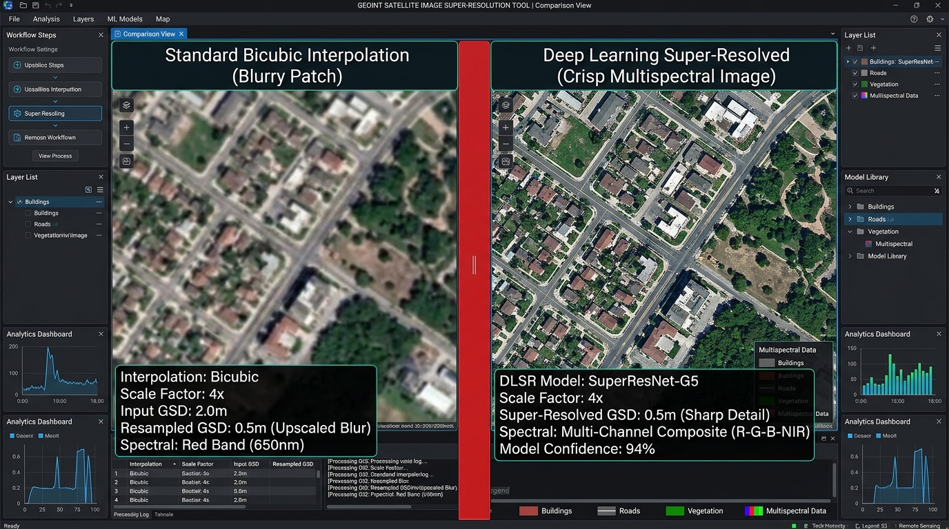
Traditional resampling techniques—such as nearest-neighbor, bilinear, or bicubic interpolation—merely smooth pixel boundaries. They interpolate pixel values without recovering genuine sub-pixel spatial details, often introducing blurring that obscures fine urban structures, narrow riparian corridors, or fragmented agricultural field boundaries.
Super-Resolution Sentinel-2 Deep Learning Remote Sensing bridges this gap by leveraging advanced Single Image Super-Resolution (SISR) neural networks, such as Enhanced Deep Residual Networks (EDSR) and Super-Resolution Generative Adversarial Networks (SRGANs). By learning complex non-linear mappings from low-resolution (LR) inputs to high-resolution (HR) ground-truth counterparts, these models upscale $10\text{ m}$ bands into finer spatial grids (e.g., $2.5\text{ m}$ or $5\text{ m}$) while preserving critical radiometric and spectral integrity.
Workflow Implementation
Deploying a deep learning super-resolution pipeline for multispectral satellite imagery requires a disciplined, end-to-end engineering workflow: data acquisition, patch pair preparation, neural network training, and rigorous spectral validation.
1. Downloading Multispectral Sentinel-2 Bands (B2, B3, B4, B8)
To feed our deep learning pipeline, we must acquire surface reflectance (Level-2A) products. Using the Google Earth Engine (GEE) Python API or direct STAC API downloads, we can extract cloud-masked chips for specific regions of interest.
For broader temporal modeling strategies, you can integrate these extraction routines with our guide on Google Earth Engine time-series analysis workflows.
Python
import ee
# Initialize the Earth Engine API
ee.Initialize()

# Define Region of Interest (ROI) and date range
roi = ee.Geometry.Polygon([[[36.7, -1.3], [37.1, -1.3], [37.1, -1.7], [36.7, -1.7]]])
collection = (
    ee.ImageCollection("COPERNICUS/S2_SR_HARMONIZED")
    .filterBounds(roi)
    .filterDate("2025-01-01", "2025-12-31")
    .filter(ee.Filter.lt("CLOUDY_PIXEL_PERCENTAGE", 10))
)

# Select 10m bands: B2 (Blue), B3 (Green), B4 (Red), B8 (NIR)
image = collection.median().select(["B2", "B3", "B4", "B8"]).clip(roi)

# Export or process raster chips locally using geemap or rasterio
2. Preparing Low-Resolution and High-Resolution Patch Pairs
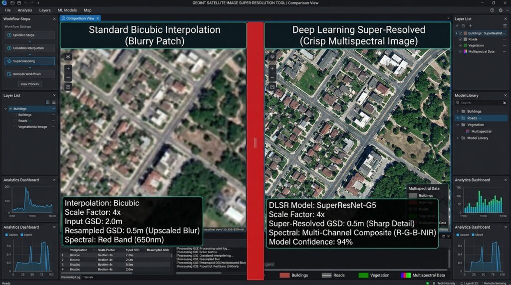
Training a supervised super-resolution network requires paired Low-Resolution ($LR$) and High-Resolution ($HR$) image patches. Following standard practice in SISR literature, we use original $10\text{ m}$ Sentinel-2 bands as our target High-Resolution ($HR$) images. We then generate corresponding Low-Resolution ($LR$) inputs by applying a Gaussian blur filter and downsampling the images by a scaling factor ($s = 2$ or $s = 4$) via bicubic degradation.
Python
import os
import numpy as np
import rasterio
from skimage.transform import resize

def create_lr_hr_pairs(input_ortho_path, hr_patch_dir, lr_patch_dir, patch_size=256, scale=4):
    os.makedirs(hr_patch_dir, exist_ok=True)
    os.makedirs(lr_patch_dir, exist_ok=True)

    with rasterio.open(input_ortho_path) as src:
        meta = src.meta.copy()
        img = src.read() # Shape: (C, H, W)
        _, height, width = img.shape

        patch_id = 0
        for y in range(0, height - patch_size + 1, patch_size):
            for x in range(0, width - patch_size + 1, patch_size):
                # Extract HR patch
                hr_patch = img[:, y:y+patch_size, x:x+patch_size]

                # Skip patches with excessive nodata/clouds
                if np.all(hr_patch == 0):
                    continue

                # Generate LR patch by downscaling
                lr_size = patch_size // scale
                lr_patch = np.zeros((hr_patch.shape[0], lr_size, lr_size), dtype=np.float32)
                for c in range(hr_patch.shape[0]):
                    lr_patch[c] = resize(
                        hr_patch[c],
                        (lr_size, lr_size),
                        order=3,
                        anti_aliasing=True
                    )

                # Save patches as numpy arrays or GeoTIFFs
                np.save(os.path.join(hr_patch_dir, f"hr_{patch_id}.npy"), hr_patch)
                np.save(os.path.join(lr_patch_dir, f"lr_{patch_id}.npy"), lr_patch)
                patch_id += 1
3. Deploying Deep Learning Super-Resolution Architectures
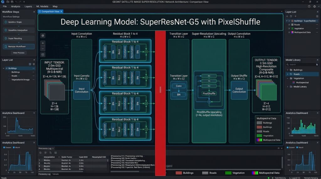
When building a neural network to upscale Sentinel 2 imagery neural network architectures, residual blocks and sub-pixel convolution layers (PixelShuffle) are preferred over traditional transposed convolutions to avoid checkerboard artifacts. Below is a PyTorch implementation of a lightweight Residual Super-Resolution block structure suited for multispectral raster processing (
Satellite image super resolution Python).Python
import torch
import torch.nn as nn
import torch.nn.functional as F

class ResidualBlock(nn.Module):
    def __init__(self, channels):
        super(ResidualBlock, self).__init__()
        self.conv1 = nn.Conv2d(channels, channels, kernel_size=3, padding=1)
        self.bn1 = nn.BatchNorm2d(channels)
        self.relu = nn.ReLU(inplace=True)
        self.conv2 = nn.Conv2d(channels, channels, kernel_size=3, padding=1)
        self.bn2 = nn.BatchNorm2d(channels)

    def forward(self, x):
        residual = x
        out = self.relu(self.bn1(self.conv1(x)))
        out = self.bn2(self.conv2(out))
        out += residual
        return out

class SatelliteSRNet(nn.Module):
    def __init__(self, in_channels=4, num_features=64, num_blocks=8, scale_factor=4):
        super(SatelliteSRNet, self).__init__()
        self.initial_conv = nn.Conv2d(in_channels, num_features, kernel_size=3, padding=1)

        # Residual blocks backbone
        self.res_blocks = nn.Sequential(*[ResidualBlock(num_features) for _ in range(num_blocks)])
        self.mid_conv = nn.Conv2d(num_features, num_features, kernel_size=3, padding=1)

        # Upsampling via PixelShuffle for 4x scaling
        self.upsample = nn.Sequential(
            nn.Conv2d(num_features, num_features * (scale_factor ** 2), kernel_size=3, padding=1),
            nn.PixelShuffle(scale_factor),
            nn.ReLU(inplace=True)
        )
        self.final_conv = nn.Conv2d(num_features, in_channels, kernel_size=3, padding=1)

    def forward(self, x):
        out1 = self.initial_conv(x)
        out = self.res_blocks(out1)
        out = self.mid_conv(out) + out1
        out = self.upsample(out)
        out = self.final_conv(out)
        return out
4. Validating Spectral Fidelity and Hallucination Checks
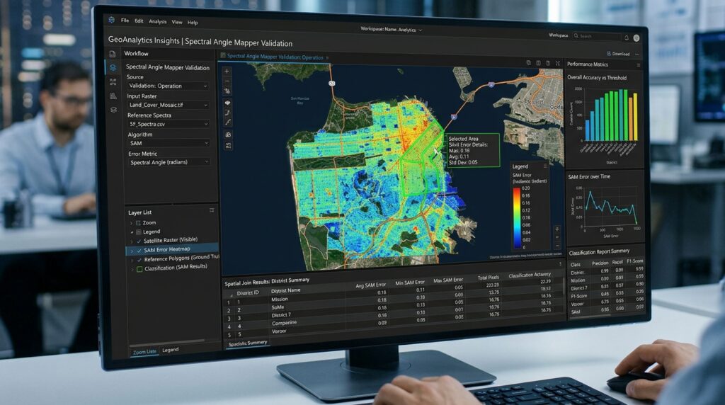
A central challenge in remote sensing super-resolution is preventing the neural network from “hallucinating” false spatial structures (e.g., inventing buildings or roads that do not exist in the physical terrain). Unlike natural RGB photographs where aesthetic sharpness is prioritized, satellite imagery demands strict radiometric and spectral consistency for downstream GIS applications like land-cover classification and change detection.
We evaluate performance using quantitative mathematical metrics:
-
Peak Signal-to-Noise Ratio (PSNR): Measures reconstruction quality of pixel intensities.
-
Structural Similarity Index (SSIM): Evaluates structural luminance, contrast, and structural preservation.
-
Spectral Angle Mapper (SAM): Calculates the spectral angle between the spectral vectors of the super-resolved pixel$$\hat{x}$$and the reference pixel$$x$$:
$$\text{SAM} = \arccos \left( \frac{\langle x, \hat{x} \rangle}{\Vert{}x\Vert{}_2 \Vert{}\hat{x}\Vert{}_2} \right)$$
To better understand how multispectral super-resolution compares against high-dimensional analytical frameworks, explore our comparative analysis on hyperspectral vs. multispectral remote sensing data processing.
Python
import numpy as np

def calculate_metrics(hr_image, sr_image):
    # Mean Squared Error
    mse = np.mean((hr_image - sr_image) ** 2)
    if mse == 0:
        psnr = float('inf')
    else:
        max_pixel = 1.0
        psnr = 20 * np.log10(max_pixel / np.sqrt(mse))

    # Spectral Angle Mapper (SAM) calculation across channels
    dot_product = np.sum(hr_image * sr_image, axis=0)
    norm_hr = np.linalg.norm(hr_image, axis=0)
    norm_sr = np.linalg.norm(sr_image, axis=0)

    # Avoid division by zero
    epsilon = 1e-8
    cos_angle = dot_product / ((norm_hr * norm_sr) + epsilon)
    cos_angle = np.clip(cos_angle, -1.0, 1.0)
    sam_rad = np.arccos(cos_angle)
    mean_sam_deg = np.mean(np.rad2deg(sam_rad))

    return {"PSNR": psnr, "Mean_SAM_Degrees": mean_sam_deg}
Summary
Enhancing open-source constellations through deep learning unlocks high-definition analytics without incurring the prohibitive costs of commercial very-high-resolution (VHR) tasking. By carefully formulating training data pipelines, building residual convolutional networks with PixelShuffle upscaling, and validating outputs using rigorous metrics like SAM and PSNR, geospatial engineers can reliably upscale $10\text{ m}$ Sentinel-2 bands into precision mapping grids tailored for modern GIS applications.