
Urban Heat Island Mapping: Calculating Land Surface Temperature (LST) from Landsat TIR Bands
1. Introduction: Mapping Urban Heat Islands with Landsat
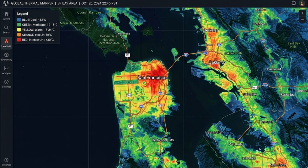
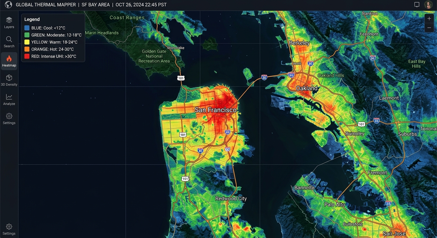
This Urban Heat Island Mapping Landsat LST Tutorial explores how built-up areas exhibit higher temperatures than their surrounding rural or less-developed environments. Urban Heat Islands (UHIs) occur when built-up areas exhibit higher temperatures than their surrounding rural or less-developed environments. Asphalt roads, concrete buildings, rooftops, and industrial surfaces absorb and store incoming solar energy, while reduced vegetation limits evaporative cooling. These conditions can create localized thermal hotspots that influence energy demand, outdoor comfort, and urban environmental planning.
Remote sensing provides an effective way to map these patterns across an entire city. Landsat 8 and Landsat 9 carry the Thermal Infrared Sensor (TIRS), which measures emitted thermal radiation in two bands. These observations can be processed to estimate Land Surface Temperature (LST), revealing spatial variations between dense urban development, parks, water bodies, and vegetated outskirts.
A critical distinction is that LST is not the same as air temperature. Air temperature describes the temperature of the surrounding atmosphere, commonly measured in a shaded, ventilated screen. LST represents the radiometric temperature of the land surface observed by the satellite. A hot roof may have a substantially higher LST than the air temperature measured nearby.
Consequently, a Landsat-derived UHI map is primarily a map of the surface urban heat island, not a direct map of pedestrian-level air temperature or human heat stress.
This tutorial demonstrates how to calculate LST in QGIS using Landsat thermal infrared bands, radiometric calibration, vegetation indices, and emissivity correction. It also explains when a manually implemented algorithm is appropriate and when using the USGS-preprocessed surface-temperature product is the more defensible choice.
2. Data Acquisition and Requirements
Landsat 8/9 bands and spatial resolution
Landsat 8 and Landsat 9 combine the Operational Land Imager (OLI), which records reflected solar radiation, with TIRS, which records thermal infrared radiation.
| Band | Sensor | Main purpose | Native spatial resolution |
|---|---|---|---|
| Band 4 | OLI | Red reflectance for NDVI | 30 m |
| Band 5 | OLI | Near-infrared reflectance for NDVI | 30 m |
| Band 10 | TIRS | Primary thermal input for single-channel LST | 100 m |
| Band 11 | TIRS | Second thermal channel for specialized retrievals | 100 m |
Although Landsat thermal data are distributed on a 30 m grid in standard products, the native thermal spatial resolution is approximately 100 m. Resampling the raster to 30 m does not create new thermal detail. This distinction matters when interpreting small roofs, narrow roads, or individual urban parcels. (USGS: Landsat band designations)
Download the imagery
Use USGS EarthExplorer or the USGS Landsat data access portal to obtain Landsat Collection 2 data.
For a manual calculation, download a matching Level-1 scene containing Band 10, the optical bands, and the MTL metadata file. For NDVI, obtain compatible optical surface-reflectance data from the same acquisition.
For most applied projects, downloading the corresponding Collection 2 Level-2 Surface Temperature product is preferable. It includes the ST_B10 layer, which has already undergone the USGS surface-temperature retrieval workflow.
The Copernicus Data Space Ecosystem is particularly useful when incorporating Sentinel imagery as a complementary data source, but USGS is the recommended primary archive for Landsat scenes.
Software requirements
Use a recent QGIS release with the built-in Raster Calculator and GDAL processing tools. Extract the downloaded Landsat files into a working directory, retaining the original band files and metadata.
Before processing, verify that all rasters cover the same scene, use compatible grids, and have the expected coordinate reference system. Do not mix scenes from different dates simply because their filenames refer to the same city.
3. Step-by-Step Workflow in QGIS
There are two practical approaches.
- Recommended operational method: Convert the existing Collection 2 Level-2
ST_B10values to degrees Celsius. - Manual retrieval method: Start with Level-1 thermal data, calculate radiance and brightness temperature, estimate emissivity, and apply a documented LST algorithm.
The first method is easier to reproduce and generally preferable for operational heat mapping. The second is useful for understanding thermal remote sensing and evaluating alternative retrieval algorithms.
Step 1: Convert thermal Digital Numbers to TOA spectral radiance
Landsat Level-1 thermal images contain calibrated digital numbers (DNs). These values must be converted into top-of-atmosphere spectral radiance before brightness temperature can be calculated.
The relationship is:
[
L_\lambda=M_LQ_{\mathrm{cal}}+A_L
]
Where:
- (L_\lambda) is spectral radiance in (\mathrm{W,m^{-2},sr^{-1},\mu m^{-1}}).
- (M_L) is the multiplicative radiance scaling factor.
- (Q_{\mathrm{cal}}) is the observed DN.
- (A_L) is the additive radiance scaling factor.
Both coefficients are supplied in the scene’s MTL metadata file. For Band 10, locate RADIANCE_MULT_BAND_10 and RADIANCE_ADD_BAND_10.
In QGIS:
- Load the Band 10 raster.
- Open Raster → Raster Calculator.
- Enter an expression using the coefficients from your own metadata file.
("B10@1" * RADIANCE_MULT_BAND_10)
+ RADIANCE_ADD_BAND_10
Replace the placeholders with numerical coefficient values. For example, if your metadata lists a multiplicative factor of 0.0003342 and an additive factor of 0.1, the expression becomes:
("B10@1" * 0.0003342) + 0.1The example coefficients are illustrative; always use the values associated with your actual scene.
Save the output as TOA_Radiance_B10.tif, keeping its extent, alignment, and CRS consistent with the source.
The USGS explains this conversion and the relevant metadata coefficients in its Level-1 data processing documentation.
Step 2: Convert spectral radiance to brightness temperature
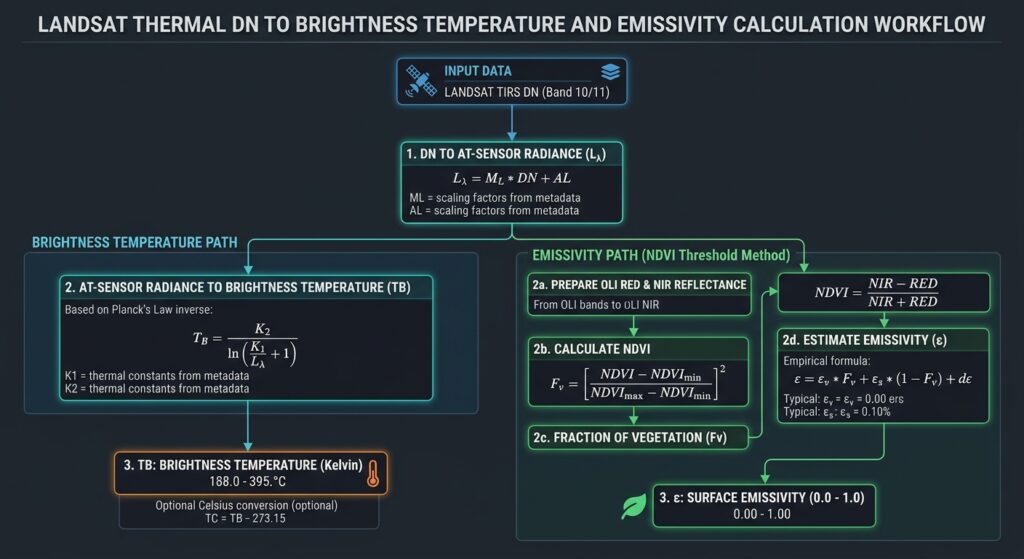
Brightness temperature represents the blackbody-equivalent temperature associated with the observed radiance. It is an intermediate quantity rather than the final land surface temperature.
The conversion uses the inverse Planck relationship:
[
BT=\frac{K_2}
{\ln\left(\frac{K_1}{L_\lambda}+1\right)}
]
Where (K_1) and (K_2) are the band-specific thermal calibration constants from the MTL file.
For Band 10, retrieve K1_CONSTANT_BAND_10 and K2_CONSTANT_BAND_10.
In the QGIS Raster Calculator:
K2 / ln((K1 / "TOA_Radiance_B10@1") + 1)Substitute the actual values for K1 and K2. Save the raster as Brightness_Temperature_K.tif.
Convert the brightness temperature from Kelvin to Celsius with:
"Brightness_Temperature_K@1" - 273.15This produces top-of-atmosphere brightness temperature in degrees Celsius. It is not yet a complete atmospheric- and emissivity-corrected LST product.
Step 3: Calculate NDVI and fractional vegetation cover
Vegetation affects surface heating through shading and evapotranspiration. NDVI provides a useful indicator of vegetation cover:
[
NDVI=\frac{NIR-Red}{NIR+Red}
]
For Landsat 8/9, use Band 5 for near-infrared and Band 4 for red reflectance.
If using Collection 2 Level-2 surface reflectance, first apply the published scaling relationship:
[
\rho=DN(0.0000275)-0.2
]
For example, calculate the scaled near-infrared raster in QGIS:
("SR_B5@1" * 0.0000275) - 0.2Then calculate scaled red reflectance:
("SR_B4@1" * 0.0000275) - 0.2Finally, calculate NDVI using the resulting reflectance rasters:
("NIR_Reflectance@1" - "Red_Reflectance@1")
/
("NIR_Reflectance@1" + "Red_Reflectance@1")
Use the actual output layer names in your project. Mask fill values, clouds, cloud shadows, and other unsuitable pixels before calculating the index. Landsat’s QA_PIXEL band contains bit-packed quality information for this purpose. The USGS documents these flags in its Collection 2 QA band reference.
Next, estimate fractional vegetation cover ((P_v)):
[
P_v=
\left(
\frac{NDVI-NDVI_{\min}}
{NDVI_{\max}-NDVI_{\min}}
\right)^2
]
A frequently used illustrative threshold pair is (NDVI_{\min}=0.2) for sparse vegetation or bare surfaces and (NDVI_{\max}=0.5) for dense vegetation.
The thresholds should be adjusted to the scene’s vegetation distribution and land-cover characteristics. Avoid accepting fractions below zero or above one.
In QGIS, use the Raster Calculator:
if(
  "NDVI@1" <= 0.2,
  0,
  if(
    "NDVI@1" >= 0.5,
    1,
    (("NDVI@1" - 0.2) / 0.3)^2
  )
)
Save this as Fractional_Vegetation.tif. This is an empirical fractional-cover estimate rather than a direct measurement of the physical fraction of vegetation within every pixel.
Step 4: Estimate land surface emissivity
Land surface emissivity ((\epsilon)) describes how effectively a surface emits thermal radiation relative to a blackbody at the same temperature. Different urban materials and natural surfaces can have different emissivities, influencing the relationship between measured radiance and actual surface temperature.
A commonly used NDVI-based approximation is:
[
\epsilon=0.004P_v+0.986
]
This approximation assigns emissivity of approximately 0.986 to bare or sparsely vegetated pixels and increases it with fractional vegetation cover. It is a simplified empirical assumption, not a universal emissivity model for all roofs, asphalt mixtures, water, soil types, and building materials.
In the QGIS Raster Calculator:
0.004 * "Fractional_Vegetation@1" + 0.986Save the result as Surface_Emissivity.tif.
For a research-grade thermal study, consider a more appropriate emissivity dataset or land-cover-specific emissivity assumptions. The USGS Collection 2 retrieval uses ASTER Global Emissivity Database information alongside NDVI and atmospheric inputs, illustrating why a single NDVI-based formula should be treated as an approximation.
Step 5: Calculate land surface temperature
There is no single universal formula that can produce a fully corrected LST raster from brightness temperature and vegetation cover alone. The appropriate method depends on the atmospheric information available and the desired accuracy.
Option A: Simplified emissivity-corrected single-channel estimate
For an exploratory workflow, a commonly used emissivity correction is:
[
LST_K=
\frac{BT_K}
{1+\left(\frac{\lambda BT_K}{\rho}\right)
\ln(\epsilon)}
]
Where:
- (BT_K) is brightness temperature in Kelvin.
- (\lambda) is the effective wavelength of Band 10, approximately (10.895,\mu m).
- (\rho=hc/k) is approximately (14380,\mu m,K).
- (\epsilon) is estimated surface emissivity.
In the Raster Calculator:
"Brightness_Temperature_K@1"
/
(
  1
  +
  (
    10.895 * "Brightness_Temperature_K@1" / 14380
  )
  * ln("Surface_Emissivity@1")
)
Convert the result to degrees Celsius:
"LST_Emissivity_Corrected_K@1" - 273.15This approach corrects for emissivity under simplifying assumptions, but it does not explicitly correct for atmospheric absorption and emission. It should therefore be described as an approximate emissivity-corrected temperature estimate, not as a complete atmospheric-corrected surface-temperature retrieval.
Option B: Full mono-window algorithm
A more rigorous single-channel approach explicitly incorporates atmospheric transmittance and an effective mean atmospheric temperature.
A widely used form is:
[
T_s=
\frac{
a(1-C-D)+
[b(1-C-D)+C+D]T_b-DT_a
}{C}
]
Where:
[
C=\epsilon\tau
]
[
D=(1-\tau)[1+(1-\epsilon)\tau]
]
Here, (T_s) is the estimated surface temperature in Kelvin, (T_b) is brightness temperature, (\epsilon) is emissivity, (\tau) is atmospheric transmittance, and (T_a) is effective mean atmospheric temperature. The coefficients (a) and (b) depend on the selected Landsat algorithm and its parameterization.
To implement this method in QGIS, prepare aligned rasters or constant rasters for the atmospheric parameters, calculate (C) and (D), and apply the equation in the Raster Calculator. Choose coefficients from a documented algorithm validated for the sensor and applicable temperature range; do not copy coefficients from a different sensor or study without checking their assumptions.
The mono-window method is more demanding than the simplified emissivity correction because accurate atmospheric parameters must be obtained from suitable profiles or a defensible retrieval method.
What about the split-window algorithm?
A split-window approach uses both thermal channels, typically Bands 10 and 11 for Landsat 8/9, to reduce atmospheric effects using the different absorption characteristics of the two bands. However, this requires an appropriate sensor-specific algorithm, calibration assumptions, and often atmospheric water-vapor information. Band 11 also has a documented calibration history that warrants care when selecting published algorithms.
For general urban heat mapping, use a validated single-channel method or the supplied Level-2 surface-temperature product rather than assuming that a generic Band 10/Band 11 expression will automatically improve accuracy.
[Image 1 placeholder: Landsat Band 10 raw scene vs resulting Land Surface Temperature map]
Alt text: “Choropleth comparison map of raw Landsat Band 10 thermal radiance versus converted Land Surface Temperature in degrees Celsius showing urban heat island hotspots.”
[Image 2 placeholder: Raster Calculator workflow flow chart for LST conversion]
Alt text: “Flowchart diagram illustrating mathematical steps to convert Landsat thermal digital numbers into brightness temperature, emissivity, and final land surface temperature.”
Step 6: The recommended shortcut — use USGS Collection 2 Level-2 surface temperature
For many applied GIS projects, the most defensible starting point is the official ST_B10 raster. This product already incorporates a more comprehensive retrieval procedure using thermal observations, emissivity information, and atmospheric inputs. See the USGS Collection 2 Level-2 Science Products documentation.
Load ST_B10 into QGIS and first mask its fill pixels. Collection 2 Level-2 surface temperature has a fill value of zero. Convert valid pixels to Kelvin using:
[
T_K=DN(0.00341802)+149
]
Then convert Kelvin to Celsius:
[
T_C=DN(0.00341802)+149-273.15
]
In the Raster Calculator:
("ST_B10@1" * 0.00341802) + 149 - 273.15Ensure that zero-valued fill pixels are excluded rather than interpreted as physical temperatures. The USGS scaling guide documents these coefficients.
The resulting raster is a more appropriate operational basis for UHI mapping than an emissivity-only correction, although it still requires examination of cloud contamination, quality flags, retrieval gaps, and known product limitations.
4. Applied Analysis: Classifying Heat Zones
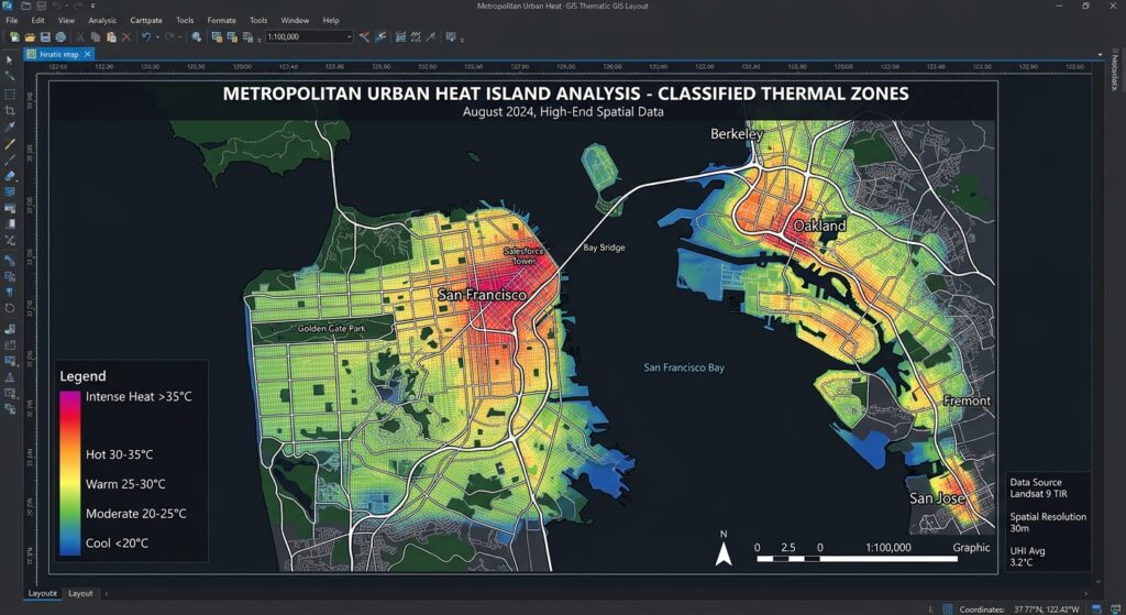
Once the LST raster is ready, style it in QGIS using Singleband pseudocolor. Choose a perceptually clear ramp that progresses from cool to warm colors and use consistent ranges when comparing different dates.
For a single-scene analysis, classify temperature into relative thermal zones. One possible standard-deviation approach is:
| Relative class | Example definition |
|---|---|
| Cooler than typical | LST below (\mu-\sigma) |
| Moderate | LST from (\mu-\sigma) to (\mu) |
| Warm | LST from (\mu) to (\mu+\sigma) |
| Hotspot | LST above (\mu+\sigma) |
Here, (\mu) is the mean LST for the valid study area and (\sigma) is its standard deviation. These are relative statistical classes, not universal health-risk thresholds. They also depend on the area included in the statistics, so document whether the summary covers the urban core, the entire scene, or a defined study boundary.
For a more direct surface urban heat-island indicator, compare average LST in the built-up area with an appropriate rural or vegetated reference zone:
\overline{T}_{\mathrm{reference}}
]
A positive value indicates that the urban surface is warmer than the chosen reference for that acquisition. It does not, by itself, establish a corresponding air-temperature difference.
Link hotspots to vegetation and built surfaces
Overlay the LST map with NDVI, land-cover classifications, or canopy-cover data to investigate whether hotter pixels tend to have lower vegetation cover.
You can also summarize temperature by administrative wards or land-use categories using zonal statistics. This allows an analyst to compare average LST across residential, industrial, commercial, and park areas.
Use comparable acquisition dates, cloud masks, spatial resolutions, and processing methods when examining patterns over time. Differences in season, antecedent rainfall, surface moisture, and acquisition time can affect LST as much as changes in urban form.
5. Quality Control and Interpretation
Before producing a final UHI map, check for the following:
Clouds and shadows: Mask them using quality flags. Cloud-contaminated thermal values should not be treated as valid surface temperatures.
Spatial resolution: Do not interpret resampled 30 m thermal pixels as independent 30 m thermal measurements. The native TIRS resolution is approximately 100 m.
Atmospheric correction: Distinguish brightness temperature, emissivity-adjusted estimates, and fully corrected surface-temperature products in your methodology.
Surface emissivity: NDVI-based emissivity is an approximation and can be unsuitable for certain urban materials. State the formula and thresholds used.
Comparison dates: Use consistent seasons and similar atmospheric conditions for change detection wherever possible.
Validation: Where available, compare the results with reliable ground measurements or independently processed temperature products, while recognizing that satellite overpass time and measurement footprints may differ from field observations.
6. SEO Best Practices and Related Tutorials
For a connected GIS learning resource, link this article to complementary technical guides:
- Calculating NDVI from Landsat imagery
- Remote sensing band combinations for land-cover interpretation
- Spatial statistics and hotspot analysis in QGIS
Replace these example paths with the canonical URLs on your website. Use descriptive anchor text and retain the main keyword in the title, introduction, and page metadata without repeating it unnaturally.
For authoritative technical references, consult the USGS Landsat TIRS and calibration documentation, the Collection 2 Surface Temperature documentation, and the USGS Landsat Level-1 conversion guide.
7. Conclusion and Key Takeaways
Landsat-based urban heat-island mapping combines thermal infrared observations with surface emissivity, vegetation information, and careful GIS processing. QGIS provides the raster tools needed to calculate radiance, brightness temperature, NDVI, fractional vegetation cover, and temperature maps, while Landsat Collection 2 Level-2 products provide a practical, preprocessed alternative.
The most important distinction is between a simplified emissivity correction and a fully corrected LST retrieval. A scientifically defensible workflow should use a documented algorithm, appropriate atmospheric information, cloud and quality masking, and clear reporting of spatial-resolution limitations.
For routine urban heat analysis, start with the USGS ST_B10 surface-temperature product, convert it using the documented scale factor and offset, and classify thermal zones relative to a clearly defined study area. Use the manual Band 10 workflow when you need to understand, reproduce, or compare the retrieval process.
A well-documented LST map can help identify potential surface heat hotspots, evaluate associations with vegetation and built-up cover, and support urban greening and climate-adaptation planning—without confusing satellite-measured surface temperature with air temperature or direct human heat exposure.