
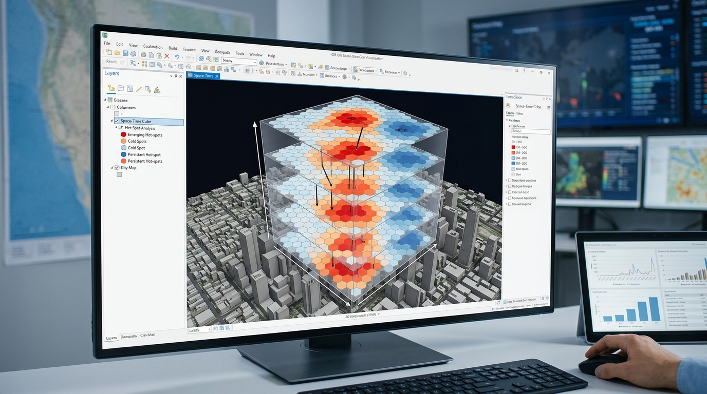
Space-Time Pattern Mining: Creating and Analyzing 3D Space-Time Cubes
1. Introduction: Moving beyond static maps
When implementing space time pattern mining 3D space time cubes, traditional maps often conceal how geographic patterns develop over time. Traditional GIS maps show where events occur, but a static map can conceal how geographic patterns develop over time. A citywide crime map, for example, may reveal concentrations of incidents without showing whether those concentrations are newly emerging, persistent, weakening, or moving between neighborhoods.
Space-time pattern mining addresses this limitation by integrating spatial location and temporal information into a structured analytical framework. Instead of treating every event as an independent point on a two-dimensional map, it aggregates observations into spatial and temporal units, allowing patterns to be evaluated across both dimensions.
The central concept is a space-time cube, in which the horizontal axes represent geographic location and the third dimension represents time:
Here, \(X\) and \(Y\) represent projected geographic coordinates, while \(T\) represents successive time intervals. Unlike a physical elevation axis, the vertical dimension represents temporal progression.
A cube can contain monthly crime counts, quarterly disease cases, annual environmental measurements, or other variables recorded consistently across geographic locations and time steps. ArcGIS Pro stores these structured observations in a NetCDF data structure that supports statistical analysis and two- or three-dimensional visualization.
1.1 Why space-time analysis matters
Consider a public-safety analyst studying residential burglaries across a city over ten years. A conventional hotspot analysis might identify neighborhoods with concentrated burglaries during the entire study period. It cannot, by itself, explain the sequence of changes that produced the final pattern.
Space-time pattern mining can distinguish between neighborhoods where hotspots are newly appearing, remaining persistent, intensifying, or diminishing. Similar methods can be used to examine disease incidence, traffic collisions, wildfires, and environmental change.
The four core concepts are:
-
Spatial aggregation: Group observations into regular grid cells, hexagons, or predefined geographic locations.
-
Temporal aggregation: Group observations into consistent intervals, such as weeks, months, quarters, or years.
-
Spatial-temporal statistical analysis: Test whether observations form statistically significant clusters and whether those clusters change over time.
-
Pattern classification: Assign meaningful categories to the temporal behavior of hotspots and cold spots.
These operations allow researchers to move from the question “Where are events concentrated?” to the more informative questions “Where are concentrations emerging, how persistent are they, and how are they changing?”
1.2 Understanding the structure of a space-time cube
A space-time cube is composed of individual space-time bins. Each bin corresponds to one spatial location and one temporal interval.
Conceptual space-time cube
Figure 1. A conceptual space-time cube. Horizontal positions represent locations; stacked layers represent successive time intervals. The colored bins are illustrative, not actual statistical results.
For a regular grid, each bin can be indexed as \(B_{i,t}\), where \(i\) identifies a spatial location and \(t\) identifies a time step. The corresponding value \(x_{i,t}\) might be the number of burglaries, mean temperature, or disease incidence count recorded for that location and period.
A complete cube provides a time series for each spatial location and a spatial snapshot for each time step. This enables analysis at two complementary scales:
-
Across time at one location: Does the variable increase, decrease, or fluctuate?
-
Across locations within a time step: Are neighboring locations experiencing unusually high or low values?
The cube does not automatically solve problems of missing observations, changing reporting practices, or population differences. Those issues must be addressed during data preparation and model design.
2. Creating the space-time cube
The workflow below uses ArcGIS Pro’s Space Time Pattern Mining toolbox. It is designed for point-event data such as reported crimes or disease cases, although space-time cubes can also be created from data organized by fixed locations or multidimensional rasters.
Step 1: Prepare and validate the input data
Before building the cube, prepare a point dataset with at least a unique identifier, valid location coordinates, and a timestamp. For an event-count analysis, one point should represent one recorded event.
For a decade-long crime analysis, a suitable input table might contain:
| Field | Example | Purpose |
|---|---|---|
Incident_ID |
CR-000145 | Unique incident identifier |
Incident_Date |
2021-07-18 | Date and time of the event |
Crime_Type |
Burglary | Optional analytical filter |
X, Y |
Projected coordinates | Incident location |
Neighborhood |
District 04 | Optional administrative reference |
Check the following before processing:
-
Remove exact duplicates and resolve records with invalid or missing timestamps.
-
Confirm that coordinates represent the correct location and coordinate reference system.
-
Use a projected coordinate system appropriate for the study region so distance intervals are measured meaningfully.
-
Establish a consistent temporal coverage and decide how incomplete periods will be handled.
-
Define the outcome being analyzed: raw counts, an aggregated attribute, or a rate derived using an appropriate exposure denominator.
Important: Event counts and event rates answer different questions. A neighborhood with more residents or more time spent in public spaces may have more incidents even when individual risk is lower. If the research question concerns risk, consider calculating defensible rates or modeling exposure rather than treating raw counts as direct measures of risk.
Step 2: Choose the spatial and temporal bins
The spatial interval determines the size of the grid cells. The temporal interval determines the duration represented by each time step.
For example, a 10-year study could use monthly intervals, giving approximately 120 time steps, or quarterly intervals, giving approximately 40 time steps. Annual intervals yield only 10 steps over a ten-year period.
Finer temporal intervals can reveal short-lived changes but often produce many zero-count bins and more unstable patterns. Coarser intervals provide more observations per bin but can conceal seasonal and short-term dynamics.
Likewise, smaller spatial cells preserve local variation but produce sparse counts; larger cells stabilize counts but may merge distinct local patterns. Choose the binning scheme according to the research objective, spatial scale, event frequency, and statistical requirements—not solely to make the output appear detailed.
Step 3: Create the cube in ArcGIS Pro
For timestamped incident points, use Create Space Time Cube By Aggregating Points.
Navigate to:
Analysis → Tools → Space Time Pattern Mining → Create Space Time Cube By Aggregating Points
The essential parameters are:
| Parameter | Example setting | Purpose |
|---|---|---|
| Input Features | Crime incident points | Source observations |
| Output Space Time Cube | Crime_Monthly.nc |
NetCDF output |
| Time Field | Incident_Date |
Timestamp of each event |
| Time Step Interval | 1 Months |
Monthly aggregation |
| Distance Interval | 400 Meters |
Spatial cell size |
| Aggregation Shape Type | Hexagon grid | Spatial bin geometry |
| Summary Fields | Optional | Statistics for numeric attributes |
The values above are an illustrative starting configuration for a city-scale analysis, not universal defaults. ArcGIS Pro requires a suitable timestamp field and projected data for distance-based cube construction; point aggregation also has minimum-data and time-step requirements.
Choose fishnet grid if square cells are appropriate or hexagon grid if a hexagonal neighborhood arrangement better matches the intended exploratory analysis. Use defined polygon locations instead when the research requires stable administrative units such as census tracts, wards, or police beats.
For a decade-long analysis, monthly intervals yield approximately 120 time steps, provided the observations span the full intended period. Before finalizing the parameters, check how many spatial cells will be created and whether most cells will contain useful observations.
Step 4: Handle empty bins and missing observations
An empty bin is not always evidence that zero events occurred.
For a complete crime-recording system, a month with no incidents in a cell may reasonably be represented by zero. But if reporting was interrupted, a clinic failed to submit disease records, or a satellite acquisition is missing, the value is unknown—not necessarily zero.
Distinguish between three conditions:
-
True zero: The process was observed and no event occurred.
-
Missing observation: The data collection process did not supply a valid measurement.
-
Estimated value: A missing bin has been filled using a documented interpolation or neighbor-based procedure.
ArcGIS Pro offers several methods for filling empty bins when summary fields are involved, including zero filling, neighbor-based estimates, and temporal interpolation. The selected
For incidence counts, zero filling should be used only where a zero is substantively justified. Avoid interpolating missing records simply to produce a visually complete cube.
Run the tool and inspect the geoprocessing messages. Confirm the spatial and temporal extent, cell dimensions, number of time steps, and count distribution. These diagnostics are part of the analysis, not just processing logs.
Step 5: Visualize the cube in three dimensions
After the NetCDF cube is created, explore its structure before running hotspot classification.
In ArcGIS Pro:
-
Open Insert → New Map → New Local Scene.
-
Open the Make Space Time Cube Layer tool from the Space Time Pattern Mining toolbox.
-
Set the
.ncfile as the input and run the tool. -
Select the space-time cube layer in the Contents pane.
-
Use the space-time cube ribbon to choose the variable, display theme, time range, and other visualization settings.
The cube can be explored as stacked temporal slices, individual locations’ time series, or other display themes supported by the analyses already performed. ArcGIS Pro also provides Visualize Space Time Cube in 3D and Visualize Space Time Cube in 2D tools.
Use this step to identify unexpected gaps, abrupt changes in data coverage, and cells with many estimated values. A visually striking pattern should always be checked against the underlying counts and data-quality information.
3. Emerging Hot Spot Analysis: The statistical framework
Emerging Hot Spot Analysis (EHSA) combines two statistical ideas: local spatial clustering and temporal trend detection. The result is a classification of each analyzed location according to how its hot- or cold-spot behavior has developed through time.
ArcGIS Pro applies a space-time implementation of the Getis-Ord \(Gi^*\) statistic to assess clustering at each bin, then uses the Mann–Kendall trend test on the resulting sequence of hot-spot statistics to determine temporal behavior. The tool also applies false discovery rate (FDR) correction to the bin-level hot-spot analysis.
3.1 Getis-Ord \(Gi^*\): Detecting local clustering
The Getis-Ord \(Gi^*\) statistic evaluates whether a location and its neighbors exhibit unusually high or low values relative to the broader dataset.
For an observation \(i\), a common standardized form of the statistic is:
where:
-
\(x_j\) is the value associated with location \(j\).
-
\(w_{ij}\) is the spatial or space-time neighborhood weight.
-
\(\bar X\) is the global mean of the values.
-
\(S\) is their standard deviation.
-
\(n\) is the number of observations represented in the calculation.
This equation describes the general standardized statistic; software implementations may use specific neighborhood, weighting, and correction procedures.
The resulting \(z\)-score indicates the direction and strength of local clustering:
-
A significantly positive \(z\)-score indicates a hot spot: high values are clustered.
-
A significantly negative \(z\)-score indicates a cold spot: low values are clustered.
-
A value that is not statistically significant does not establish a local cluster.
A location with a high event count is not automatically a statistically significant hotspot. Its value must be assessed in the context of the specified neighborhood.
In space-time analysis, neighborhood definitions may incorporate spatially adjacent cells and values from earlier time steps. The neighborhood distance and temporal depth therefore influence which patterns the method detects.
3.2 Mann–Kendall: Testing temporal trends
Mann–Kendall is a nonparametric test for a monotonic trend in an ordered time series. It evaluates whether later observations tend to be greater than or less than earlier observations without requiring the series to follow a linear trend.
For a series \(x_1,\ldots,x_n\), the Mann–Kendall statistic is:
where the sign function is positive when \(x_j>x_i\), negative when \(x_j<x_i\), and zero when the values are tied.
A trend statistic and its variance are used to calculate a standardized test statistic. Appropriate implementations account for tied values, and serial dependence may also need consideration in methodological designs outside the standard tool workflow.
In a space-time cube, there are two related but distinct uses of temporal trend analysis:
-
Cube-level trend analysis: Examines how the input count or summary variable changes over time at each spatial location.
-
Emerging Hot Spot Analysis: Examines the time sequence of local \(Gi^*\) statistics to identify whether hot- or cold-spot clustering is increasing, decreasing, recurring, or persisting.
This distinction matters. An increase in raw event counts is not identical to an increase in statistically significant hotspot intensity. The latter accounts for how the location compares with its neighbors.
3.3 Understanding FDR correction
When thousands of bins are tested for spatial clustering, some may appear significant by chance. Testing many hypotheses increases the risk of false positives.
ArcGIS Pro applies false discovery rate correction in Emerging Hot Spot Analysis to adjust the interpretation of bin-level statistical significance across multiple tests. The resulting classification is therefore not simply a display of the largest counts or unadjusted \(z\)-scores.
This does not eliminate every inferential limitation. Results still depend on the input data, spatial and temporal aggregation, neighborhood definitions, and the assumptions underlying the analysis. Researchers should report these decisions, especially when outputs are used in policy or resource allocation.
3.4 Run Emerging Hot Spot Analysis
Navigate to:
Analysis → Tools → Space Time Pattern Mining → Emerging Hot Spot Analysis
Configure the tool as follows:
| Parameter | Illustrative configuration |
|---|---|
| Input Space Time Cube | Crime_Monthly.nc |
| Analysis Variable | COUNT |
| Output Features | Crime_EmergingHotspots |
| Neighborhood Distance | 800 Meters |
| Neighborhood Time Step | 1 |
| Conceptualization of Spatial Relationships | Fixed distance |
| Number of Neighbors | Optional, based on study design |
For a 400-metre cell dimension, an 800-metre neighborhood distance is a reasonable starting test for a city-scale grid, not a universal choice. Test the neighborhood against the geography and the likely mechanisms of interaction. A larger distance captures broader spatial clustering, while a smaller distance emphasizes more local patterns.
The temporal-neighborhood setting also matters: the tool can include bins from the same locations and their spatial neighbors over the specified number of prior intervals. For monthly data, a neighborhood time step of 1 examines the current interval and the previous interval in the relevant neighborhood configuration.
Run the analysis and inspect the tool messages for warnings, excluded locations, and summary statistics. Save the output feature class and retain the NetCDF cube used to produce it.
4. Interpreting Emerging Hot Spot categories
Emerging Hot Spot Analysis classifies locations into categories based on the sequence of statistically significant hot or cold spots across the time steps.
The standard ArcGIS Pro workflow identifies eight hot-spot patterns, their eight cold-spot counterparts, and a category for locations that do not fit the defined patterns. Some categories depend on whether a hotspot appears in the most recent time step, how often it has appeared, and whether its clustering intensity has a statistically significant trend.
4.1 The major hot-spot categories
| Category | Statistical interpretation | Example in crime analysis |
|---|---|---|
| New Hot Spot | Statistically significant hotspot in the final time step, with no earlier significant hotspot | A neighborhood becomes a significant burglary hotspot for the first time in the final month |
| Consecutive Hot Spot | At least two consecutive significant hotspot intervals at the end of the series, with no prior hotspot run and hotspots in fewer than 90% of all intervals | A new cluster persists over the last few months |
| Intensifying Hot Spot | Significant hotspot in at least 90% of intervals, including the final interval, with a significant increasing trend in clustering intensity | A long-standing hotspot becomes more intense |
| Persistent Hot Spot | Significant hotspot in at least 90% of intervals, with no discernible trend in clustering intensity | The hotspot remains consistently significant |
| Diminishing Hot Spot | Significant hotspot in at least 90% of intervals, including the final interval, with a significant decreasing trend in clustering intensity | A long-term hotspot weakens but remains significant |
| Sporadic Hot Spot | Significant hotspot in the final interval with an intermittent history of hotspots, fewer than 90% of intervals significant, and no prior significant cold spots | An area repeatedly becomes a hotspot but not consistently |
| Oscillating Hot Spot | Significant hotspot in the final interval and at least one prior significant cold-spot interval, with hotspots in fewer than 90% of intervals | An area alternates between significant cold and hot periods |
| Historical Hot Spot | Not a hotspot in the final interval, but statistically significant hotspot in at least 90% of the intervals | A historically persistent crime hotspot that is no longer significant |
These definitions follow the ArcGIS Pro category rules, including the 90% thresholds used for several patterns.
The cold-spot categories mirror these interpretations for statistically significant clustering of low values. For example, a new cold spot is a location that is significantly cold in the final time interval but was never a significant cold spot earlier. Historical cold spots were significant in at least 90% of intervals but are no longer significant in the latest one.
A common analytical mistake is treating these classes as simple rankings. An intensifying hotspot does not necessarily have the highest absolute crime count, and a persistent hotspot is not necessarily the most dangerous location. The classifications describe statistically significant clustering behavior relative to the specified analysis neighborhood.
4.2 Use the categories to answer specific questions
The value of the categories lies in the decisions they can support.
-
Where should new interventions be investigated? New or consecutive hotspots may warrant closer examination to determine why clustering has recently emerged.
-
Where is the pattern worsening? Intensifying hotspots indicate an increasing trend in the intensity of high-value clustering.
-
Where are long-standing patterns stable? Persistent hotspots identify locations where clustering has remained statistically significant without a discernible increasing or decreasing trend.
-
Where might conditions be improving? Diminishing hotspots indicate a statistically significant decline in clustering intensity, while historical hotspots are no longer significant in the most recent period.
-
Where is the pattern unstable? Sporadic and oscillating hotspots indicate intermittent behavior rather than consistent clustering.
These interpretations should be combined with substantive context. A classification is a statistical description of the observed pattern—not proof of causation or a recommendation for an intervention by itself.
5. Practical application: Analyzing a decade of urban crime
Consider a hypothetical city with ten years of geocoded residential burglary incidents, from January 2015 through December 2024. The objective is to identify which neighborhoods experienced newly emerging, persistent, intensifying, or diminishing burglary hotspots.
The following workflow demonstrates the complete analytical sequence.
Stage 1: Define the research design
Begin by specifying the questions before selecting spatial and temporal bin sizes.
| Research component | Example design |
|---|---|
| Study period | January 2015–December 2024 |
| Outcome | Monthly burglary incident count |
| Spatial unit | Hexagonal grid |
| Spatial bin size | 400 m, subject to sensitivity testing |
| Temporal interval | One month |
| Statistical method | Space-time \(Gi^*\) followed by Mann–Kendall trend evaluation |
| Output | Hotspot category map, time series, and 3D cube |
This design provides approximately 120 monthly observations per continuously represented spatial location. The final number of bins depends on the study extent, the spatial grid, and the source data.
Check that the event reporting system was sufficiently consistent across the ten-year period. Changes in police reporting, geocoding accuracy, crime definitions, or incident-recording systems can produce apparent temporal patterns that do not reflect actual changes in crime.
Stage 2: Create the cube and run the analysis using ArcPy
The process can be automated with ArcPy inside a compatible ArcGIS Pro Python environment. The following script illustrates the central tool calls for a projected crime-point feature class.
import arcpyimport osarcpy.env.overwriteOutput = True# Replace these paths and field names with your own.workspace = r"C:\STPM"incident_points = ( r"C:\STPM\Crime.gdb\Residential_Burglaries")time_field = "Incident_Date"cube_path = os.path.join( workspace, "Crime_Monthly_2015_2024.nc")output_gdb = os.path.join( workspace, "Results.gdb")output_hotspots = os.path.join( output_gdb, "Crime_EmergingHotspots")# Create Space Time Cube By Aggregating Points.arcpy.stpm.CreateSpaceTimeCube( in_features=incident_points, output_cube=cube_path, time_field=time_field, template_cube="#", time_step_interval="1 Months", time_step_alignment="End time", reference_time="#", distance_interval="400 Meters", summary_fields="#", aggregation_shape_type="HEXAGON_GRID",The parameter values are illustrative. The analysis extent, time alignment, neighborhood size, and grid dimensions should be adjusted to the actual data and research question. The script assumes that the input time field is a valid date field and that the feature class uses a suitable projected coordinate system.
The ArcGIS Pro geoprocessing functions and parameter patterns are documented in the Create Space Time Cube By Aggregating Points and Emerging Hot Spot Analysis references.
Run the script in an environment where ArcPy and the required ArcGIS Pro tools are available. Review the geoprocessing messages if any step fails, and confirm that the resulting cube actually spans the intended period.
Stage 3: Interpret the hotspot map
Add Crime_EmergingHotspots to an ArcGIS Pro map and inspect the output category field. Use unique-value symbology to distinguish the hotspot patterns from cold spots and locations with no detected pattern.
The initial interpretation should focus on three questions:
-
Where did clustering emerge recently? Map New and Consecutive Hot Spots to identify locations whose recent behavior differs from their earlier history.
-
Where did clustering persist or intensify? Compare Persistent and Intensifying Hot Spots to distinguish stable long-term clustering from a statistically significant increase in clustering intensity.
-
Where did historical patterns weaken or fluctuate? Investigate Diminishing, Historical, Sporadic, and Oscillating Hot Spots to distinguish weakening clusters from intermittent ones.
Then compare those patterns with explanatory variables where available, such as population density, land use, road accessibility, business activity, and changes in reporting practices. These comparisons can help generate hypotheses, but the hotspot classification itself cannot establish which factor caused the observed pattern.
Stage 4: Inspect the 3D space-time cube
Return to the NetCDF cube and visualize it in a local 3D scene. Inspect the monthly values and the hotspot results through successive intervals.
For example, a persistent hotspot might show elevated clustering across most years, while a new hotspot may appear only near the end of the observation period. The 3D representation helps researchers connect the final two-dimensional classification map to the temporal sequence that produced it.
Use Visualize Space Time Cube in 3D or Make Space Time Cube Layer to inspect the values and available analysis themes.
The visualization is a diagnostic and communication tool. The height of a cube layer represents time ordering, not physical elevation, and color represents the selected attribute or statistical result. Neither the visual appearance nor the apparent height of a bin replaces the underlying statistical test.
6. Adapting the workflow to disease outbreaks and urban heat
The same space-time framework can support several environmental and public-health applications, but the meaning of an observation and the treatment of missing values must match the phenomenon being studied.

Disease outbreak progression
Aggregate geocoded cases into weekly or monthly spatial bins. Use disease counts for event-clustering analysis, but consider population-based incidence rates or appropriate statistical models when comparing places with different population sizes. Account for reporting delays, changes in case definitions, and incomplete surveillance before interpreting new or intensifying clusters.

Urban heat island evolution
Start with consistently measured temperature observations, such as station measurements or comparable satellite-derived land surface temperature products. If observations are supplied as a multidimensional raster, ArcGIS Pro can create a space-time cube from the multidimensional raster layer. Check acquisition dates, cloud contamination, sensor consistency, and seasonal comparability before interpreting temperature trends.
In these applications, the space-time cube provides a consistent framework, but it does not eliminate the need to choose a meaningful outcome variable. Case counts, incidence rates, air temperature, and land surface temperature describe different processes and require different quality controls.
7. Statistical limitations and research safeguards
Before treating an emerging hotspot map as evidence for a decision, assess the following methodological risks.
The modifiable areal unit problem (MAUP). Results can change with the size, shape, or alignment of spatial bins. Repeat the analysis with scientifically defensible alternative grid sizes or neighborhood definitions.
Temporal aggregation effects. Monthly intervals may reveal short-lived clusters, while annual intervals may hide them. Check whether the selected time step matches the timescale of the process.
Multiple comparisons and spatial dependence. FDR correction helps control false discoveries, but it does not resolve every assumption or dependence issue. Document the significance procedure and the conceptualization of spatial relationships.
Changing exposure and reporting. Raw counts may increase because population, observation coverage, or reporting changes. Consider rates or appropriate denominators when the research question concerns risk or intensity relative to exposure.
Missing-data bias. A gap in observation is not automatically a zero. Missing values that are improperly filled can alter both the temporal trend and the hotspot classification.
Interpretation versus causation. A significant spatial-temporal pattern is not a causal explanation. Use additional data and a suitable study design to examine possible drivers.
8. Summary checklist for spatial-temporal research
Use this checklist when planning, executing, or reviewing a space-time pattern mining project.
Research quality checklist
0 / 16 complete
Data preparation
Cube design
Statistical analysis
Interpretation and reporting
9. Conclusion
Space-time pattern mining extends conventional GIS analysis by structuring observations into spatial and temporal bins, then testing how their values and clustering behavior develop over time.
The space-time cube provides the analytical structure. Getis-Ord \(Gi^*\) identifies statistically significant local clustering, while Mann–Kendall evaluates monotonic temporal trends. Emerging Hot Spot Analysis combines these components to distinguish new, consecutive, intensifying, persistent, diminishing, sporadic, oscillating, and historical hotspot patterns.
The resulting classifications can support crime analysis, disease surveillance, environmental monitoring, and urban climate research. Their reliability depends on defensible bin dimensions, appropriate temporal intervals, sound neighborhood definitions, good data quality, and careful interpretation.
The key research principle is to treat the space-time cube as a statistical model of how observations are organized—not merely as a 3D visualization. A rigorous workflow tests the sensitivity of the results, distinguishes observed changes from data artifacts, and reports the assumptions that shape the final map.
Further reading
-
ArcGIS Pro: Create Space Time Cube By Aggregating Points — cube parameters, bin dimensions, and input-data requirements.
-
ArcGIS Pro: How Emerging Hot Spot Analysis Works — category definitions, \(Gi^*\), trend tests, and neighborhoods.
-
ArcGIS Pro: Emerging Hot Spot Analysis — tool parameters, outputs, and ArcPy syntax.
-
ArcGIS Pro: Visualize the Space-Time Cube — 2D and 3D cube exploration.