Table of Contents

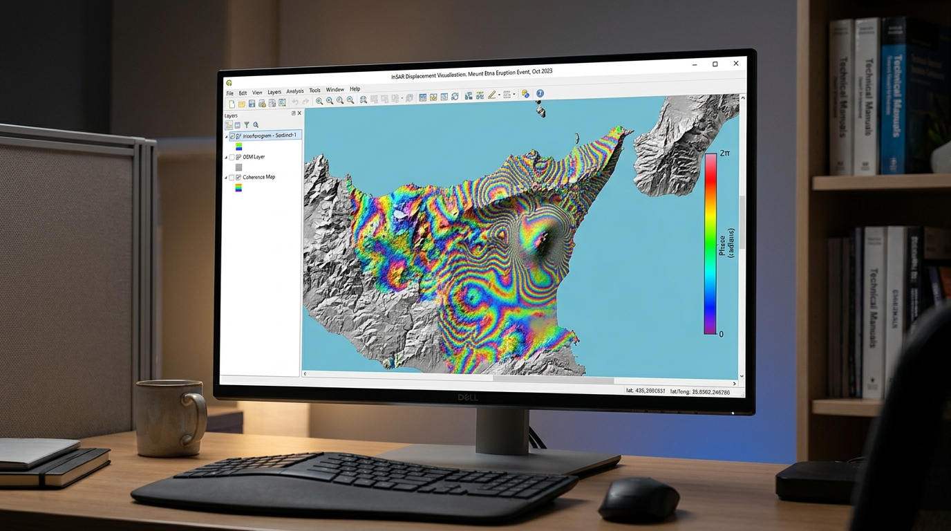
InSAR Surface Deformation Mapping: Tracking Ground Subsidence with Sentinel-1

1. Introduction: How InSAR detects ground subsidence

InSAR Surface Deformation Mapping Sentinel 1 Subsidence

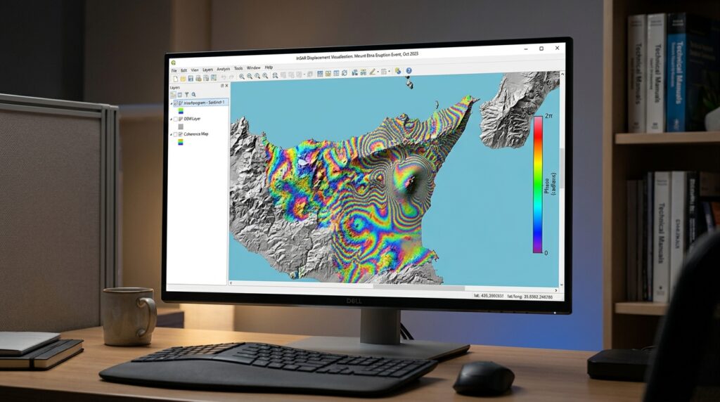
When performing InSAR surface deformation mapping Sentinel 1 subsidence, detecting millimeters of ground displacement from satellite radar requires careful processing. Interferometric Synthetic Aperture Radar (InSAR) is a remote sensing technique that measures changes in the distance between a radar satellite and the Earth’s surface by comparing the phase of radar signals acquired at different times.

Unlike optical remote sensing, Synthetic Aperture Radar (SAR) actively transmits microwave pulses and records the returning signal. This makes Sentinel-1 useful for monitoring ground deformation in areas where clouds, darkness, or frequent optical image gaps would complicate conventional satellite mapping.

InSAR surface deformation mapping with Sentinel-1 is particularly valuable for identifying gradual land subsidence associated with groundwater extraction, underground mining, urban development, and natural geological processes. It can also help monitor volcanic inflation, earthquake-related displacement, and unstable slopes.

The central principle is that a radar signal records both amplitude and phase. Amplitude describes the strength of the returning signal, while phase describes the position of the signal within its wave cycle. When two compatible radar acquisitions cover the same ground, changes in their phase can reveal subtle changes in the radar-to-ground path length.

Under favorable conditions, carefully processed InSAR observations can resolve millimeter-scale changes. That does not mean every Sentinel-1 interferogram has millimeter accuracy: coherence, atmospheric conditions, processing choices, and reference stability all affect the reliability of a measurement.

1.1 Understanding interferometric phase

A Sentinel-1 Single Look Complex (SLC) image stores complex-valued radar samples. A simplified representation of a pixel is:

\[ S=Ae^{i\phi} \]

where:

\(S\) is the complex radar signal.
\(A\) is its amplitude.
\(\phi\) is its phase, measured in radians.
\(i=\sqrt{-1}\).

Suppose two SLC acquisitions observe the same area: a master image acquired at time \(t_1\) and a secondary image acquired at time \(t_2\).

Their complex interferogram is commonly formed as:

\[ I=S_1S_2^* \]

where \(S_2^*\) is the complex conjugate of the secondary image.

The wrapped interferometric phase is:

\[ \Delta\phi_{\mathrm{wrapped}} =\arg(I) \]

This phase difference is initially restricted to a principal interval such as \([-\pi,\pi]\). It contains contributions from ground displacement, terrain elevation, atmospheric propagation delays, orbit inaccuracies, and noise.

The processing objective is to isolate the deformation-related component from these other contributions.

1.2 Converting phase into displacement

Sentinel-1 operates in the C-band, with a radar wavelength of approximately 5.6 cm. Because the radar signal travels from the satellite to the ground and back again, a change in the one-way line-of-sight distance of half a wavelength produces approximately one complete \(2\pi\) phase cycle.

After removing the modeled topographic contribution and unwrapping the phase, the line-of-sight displacement can be expressed as:

\[ d_{\mathrm{LOS}} =-\frac{\lambda}{4\pi}\Delta\phi_{\mathrm{def}} \]

where:

\(d_{\mathrm{LOS}}\) is the displacement along the satellite’s radar line of sight, in metres.
\(\lambda\) is the radar wavelength, in metres.
\(\Delta\phi_{\mathrm{def}}\) is the deformation-related unwrapped phase, in radians.

The negative sign assumes a particular master-secondary interferogram convention. Different software or image ordering can reverse the phase sign, so verify the convention before interpreting positive and negative displacement.

For a wavelength of approximately 5.6 cm, one full \(2\pi\) phase cycle represents about 2.8 cm of line-of-sight displacement. Phase unwrapping is essential when accumulated phase changes exceed one cycle.

Important distinction: InSAR measures displacement projected onto the satellite’s line of sight, not automatically vertical subsidence. Horizontal ground movement can contribute to the same measurement.

1.3 The processing workflow at a glance

1. Acquire SLC data

Select compatible Sentinel-1 acquisitions and a DEM

2. Coregister acquisitions

Orbit correction → TOPS split → Back-geocoding → ESD

3. Generate differential interferogram

Interferogram → Coherence → Topographic phase removal

4. Unwrap and calculate displacement

Phase filtering → SNAPHU → LOS displacement

5. Map and assess

Geocode → Export GeoTIFF → QGIS → Validate subsidence hotspots

Figure 1. A differential InSAR workflow for Sentinel-1 Interferometric Wide Swath (IW) TOPS data.

2. Data requirements: Sentinel-1 SLC image pairs

2.1 Download suitable Sentinel-1 acquisitions

Obtain Sentinel-1 Level-1 Single Look Complex products from the Copernicus Data Space Ecosystem data catalogue.

Open the Copernicus Data Space Ecosystem and search for products covering the area of interest. The catalogue and its OData API support searching Sentinel-1 products by acquisition time, product type, and other metadata.

For conventional land subsidence mapping, prioritize the following settings:

Selection criterion	Recommended choice
Product type	Level-1 SLC
Acquisition mode	IW (Interferometric Wide Swath), where available
Polarization	A common polarization, often VV
Orbit direction	Same ascending or descending pass
Relative orbit	Same track and acquisition geometry
Spatial coverage	Both acquisitions must cover the same target area and compatible bursts
Acquisition interval	Prefer a short temporal separation when possible
Perpendicular baseline	Prefer a sufficiently small baseline to limit geometric decorrelation and topographic sensitivity

Short temporal separation helps preserve coherence because the surface has less time to change. A smaller perpendicular baseline generally reduces geometric decorrelation and sensitivity to elevation differences. However, the best pair also depends on the landscape, acquisition geometry, and objectives; there is no single baseline threshold that works for every site.

For long-term subsidence monitoring, plan a multi-date stack rather than relying on one image pair. A pair can estimate displacement between two acquisition dates, but it cannot by itself establish whether the motion followed a steady annual trend.

2.2 Why SLC is essential

Sentinel-1 products come in different processing levels. For interferometry, SLC preserves complex phase information, whereas Ground Range Detected (GRD) products are detected products that do not retain the complex phase required for conventional interferometric processing.

An SLC product typically includes a .SAFE product directory containing measurement data and metadata. Sentinel-1 IW SLC products are the standard input for the TOPS interferometric workflow described below.

Useful official resources include the Copernicus data access documentation and the ESA SNAP tutorials.

2.3 Prepare the supporting datasets

In addition to the SLC pair, prepare:

A digital elevation model (DEM): Use a suitable source such as Copernicus DEM or SRTM to model and remove topographic phase. DEM accuracy affects the residual topographic signal.
Orbit files: Apply the best suitable orbit information available for each acquisition, typically precise orbit files when available.
A study-area boundary: Optional, but useful for subsetting the images and limiting processing costs.
A reference area or stable reference point: Needed to interpret displacement relative to a consistent location.
Independent validation data: GNSS measurements, leveling observations, or other suitable ground evidence are valuable for checking the inferred displacement.

Organize the inputs by acquisition date and preserve the original products. Avoid mixing incompatible tracks or silently changing the selected burst extent between the two acquisitions.

3. Step-by-step processing workflow in SNAP

The following procedure uses the classic Sentinel-1 IW TOPS differential InSAR workflow in ESA’s SNAP desktop application. Menu labels may vary by SNAP version; where necessary, use the operator search or Graph Builder to configure the processing chain.

Step 1: Apply orbit corrections and select matching bursts

Purpose: Improve the satellite positioning information and isolate the same ground coverage in both acquisitions.

Open SNAP and load both Sentinel-1 SLC .SAFE products using File → Open Product.
Run Radar → Apply Orbit File on each acquisition. Select the best appropriate orbit file available.
Run the TOPSAR-Split operator on both products.
Select the same subswath, such as IW2, and the same polarization, such as VV.
Select matching bursts that cover the study area. Apply the same selection to the master and secondary products.

The master provides the reference geometry. The secondary acquisition will subsequently be resampled into alignment with it.

Do not select burst ranges independently just because they cover similar-looking areas. The same radar coverage must be available in both acquisitions for valid interferometric processing.

Step 2: Coregister the SLC images

Coregistration aligns corresponding pixels from the two acquisitions. Small misalignments can contaminate the interferometric phase, so this step is particularly important for Sentinel-1 TOPS data.

In SNAP’s processing chain, use the following operators:

Back-Geocoding → Enhanced-Spectral-Diversity (ESD)

Run Back-Geocoding with the master and secondary split products.
Select an appropriate DEM for the processing area.
Confirm that the operator completes successfully and generates a coregistered product.
Run Enhanced-Spectral-Diversity on the coregistered product to estimate and correct residual azimuth misregistration between TOPS bursts.

ESD is an important part of the conventional Sentinel-1 TOPS interferometry workflow because residual azimuth misregistration can introduce phase errors at burst boundaries. ESA’s Sentinel-1 tutorial covers TOPS coregistration and the subsequent interferometric operators.

Quality check: Inspect the coregistration results before continuing. Failed ESD convergence, incompatible bursts, or poor overlap can compromise the entire deformation product.

Step 3: Generate the interferogram and coherence raster

Purpose: Calculate the wrapped phase difference and determine where the two acquisitions retain a sufficiently consistent radar signal.

Run SNAP’s Interferogram operator on the coregistered product.

Configure the available options to:

Subtract the modeled flat-earth phase.
Generate the coherence band.
Preserve the interferometric phase output.

The interferogram operator combines the complex radar observations to calculate the phase difference between the master and secondary acquisitions.

Coherence measures the consistency of the complex signals within a local estimation window. It is commonly represented by values between 0 and 1, where higher values indicate more reliable phase information and lower values indicate greater decorrelation.

Next, run TOPSAR-Deburst if your workflow requires a continuous image across the selected TOPS bursts.

Inspect both the wrapped phase and coherence layers. Coherent built-up areas may provide useful measurement points, while dense vegetation, changing agricultural fields, and water often produce less reliable phase measurements.

A wrapped interferogram should not be interpreted as a displacement map yet. Its colors represent cyclic phase values, and those values still contain topographic and other unwanted contributions.

Step 4: Remove the topographic phase

Purpose: Isolate phase variations associated with ground deformation by subtracting the phase predicted from terrain elevation and acquisition geometry.

Run SNAP’s TopoPhaseRemoval operator using the selected DEM and interferometric product.

Conceptually, the observed phase can be decomposed as:

\[ \phi_{\mathrm{obs}} =\phi_{\mathrm{flat}} +\phi_{\mathrm{topo}} +\phi_{\mathrm{def}} +\phi_{\mathrm{atm}} +\phi_{\mathrm{orb}} +\phi_{\mathrm{noise}} \]

where the terms represent flat-earth geometry, topography, deformation, atmospheric effects, orbit-related errors, and noise.

After flat-earth and modeled topographic phase corrections, the residual interferogram should primarily represent deformation, atmospheric effects, residual orbit or elevation errors, and noise.

Important: Topographic phase removal is not optional for this differential deformation workflow. Omitting it can cause terrain-related phase patterns to be mistaken for subsidence or uplift.

A higher-resolution DEM may improve the terrain representation, but DEM quality, alignment, and height reference also matter. Residual elevation errors can still generate spurious phase signals.

Step 5: Filter the phase and prepare for unwrapping

Purpose: Reduce phase noise before reconstructing a continuous phase surface.

Run SNAP’s GoldsteinPhaseFiltering operator on the differential interferogram.

Phase filtering can improve the local continuity of coherent phase patterns, but aggressive filtering may erase small-scale deformation features or smooth genuine displacement gradients.

Keep the coherence layer available so that poorly measured pixels can be excluded or flagged.

For initial investigations, a coherence threshold around 0.3–0.4 can be a useful trial setting, not a universal scientific cutoff. Select the actual threshold based on the land cover, coherence distribution, and acceptable measurement uncertainty.

Step 6: Unwrap the interferometric phase with SNAPHU

The wrapped phase only records values modulo \(2\pi\). Phase unwrapping estimates the integer number of cycles that must be added or subtracted to construct a continuous phase field.

SNAPHU is a statistical-cost, network-flow algorithm designed for two-dimensional phase unwrapping. Its statistical model and parameter configuration should reflect whether the interferogram is being processed for topography, deformation, or another application.

Install the SNAPHU plugin in SNAP if it is not already available:

Tools → Plugins → Available Plugins → SNAPHU Unwrapping

Then follow this sequence:

Run Radar → Interferometric → Unwrapping → Snaphu Export on the filtered differential interferogram.
Select the appropriate deformation processing mode where the operator offers a statistical-cost mode, and configure the output folder and other required parameters.
Run Snaphu-unwrapping using the exported input and configuration files.
Preserve the exported files and unwrapping logs.
Run Snaphu Import to bring the unwrapped result back into SNAP.

Inspect the unwrapped phase for abrupt jumps, large isolated patches, and discontinuities across low-coherence regions. Unwrapping algorithms can produce plausible-looking surfaces even when the solution is wrong, particularly where phase information is sparse or noisy.

Do not attempt to interpret disconnected, unreliable areas as measured displacement. Mask or flag those areas and document their limitations.

Step 7: Convert unwrapped phase to displacement

Once the unwrapped phase has been imported, use SNAP’s Phase to Displacement operator.

The operator converts phase to line-of-sight displacement using the radar wavelength. The output represents a relative displacement measurement between acquisitions, subject to the interferogram convention and reference choice.

For the conventional phase-to-displacement relationship:

\[ d_{\mathrm{LOS}} =-\frac{\lambda}{4\pi}\phi_{\mathrm{unwrapped}} \]

Here, the input must be the appropriate unwrapped deformation phase—not the original wrapped phase.

After conversion:

Inspect the displacement raster and its units.
Identify an appropriate stable reference location.
Reference the displacement to that location if needed.
Run Radar → Geometric → Terrain Correction → Range-Doppler Terrain Correction to geocode the displacement and coherence products.

Select the desired map CRS and pixel spacing, and export the geocoded results as GeoTIFFs.

The resulting deformation raster is a line-of-sight displacement map, not automatically a vertical elevation-change map. This distinction must remain explicit in the final GIS layer and map legend.

4. Track land subsidence in QGIS

Once the geocoded GeoTIFFs are ready, QGIS can be used to visualize displacement, calculate an indicative rate, and delineate potential subsidence hotspots.

Step 1: Load the rasters

Open QGIS and navigate to Layer → Add Layer → Add Raster Layer.

Load the following:

The geocoded LOS displacement raster.
The geocoded coherence raster.
An optional administrative boundary, groundwater extraction dataset, mine boundary, or other reference layer.

Check the raster CRS, pixel dimensions, NoData values, and reported displacement units before performing calculations.

Step 2: Calculate an annualized LOS displacement rate

A single interferometric pair measures displacement accumulated between two acquisition dates. To express that displacement as an indicative annualized rate, divide it by the time interval.

If the displacement raster stores metres, calculate:

\[ v_{\mathrm{LOS}} =\frac{100d_{\mathrm{LOS}}}{\Delta t} \times365.25 \]

where:

\(v_{\mathrm{LOS}}\) is in centimetres per year.
\(d_{\mathrm{LOS}}\) is in metres.
\(\Delta t\) is the number of days between acquisitions.

In Raster → Raster Calculator, an example for a 12-day interval is:

"displacement_m@1" * 100 * 365.25 / 12

Replace displacement_m@1 with the actual band name and 12 with the true acquisition interval in days.

This calculation assumes that the motion was approximately linear throughout the period. It does not establish a long-term annual trend from a single pair. For defensible annual velocity estimates, process a multi-date stack using a time-series method, such as Small Baseline Subset (SBAS) or Persistent Scatterer InSAR (PSInSAR), where appropriate. GMTSAR provides documented workflows for batch interferograms and SBAS time-series processing.

Step 3: Apply a coherence mask

Poor-coherence pixels should not be treated as reliable displacement measurements.

Use the coherence raster to mask low-quality areas before calculating hotspot statistics. For example, test a threshold of 0.35, inspect the resulting mask, and adjust it to match the study area’s land cover and measurement requirements.

Do not confuse a low coherence value with a subsidence signal. Coherence describes measurement reliability, not the amount of ground movement.

Step 4: Style the deformation map

In QGIS, open Layer Properties → Symbology and select a single-band pseudocolor renderer.

Use a diverging color ramp centered around zero, with one side representing motion toward the satellite and the other representing motion away from it. Confirm the processor’s sign convention before assigning those labels; do not automatically label negative values as subsidence.

Overlay roads, buildings, mine boundaries, geological units, and groundwater extraction locations where suitable data are available.

For hotspot identification, consider both the magnitude and spatial continuity of the signal. A coherent deformation bowl may be more informative than isolated extreme pixels, which can reflect phase-unwrapping errors or atmospheric artifacts.

Finally, export the styled layer or layout as a map for reporting. Keep the displacement units, acquisition dates, reference point, coherence threshold, and line-of-sight interpretation in the map metadata or accompanying notes.

5. Limitations and quality control

Limitation	Effect on the result	Recommended response
Temporal decorrelation	Surface changes between acquisitions reduce phase reliability	Prefer shorter time intervals and coherent targets
Vegetation	Changing leaves, soil moisture, and canopy structure can reduce coherence	Mask unreliable areas and consider multi-temporal approaches
Atmospheric delay	Differences in atmospheric conditions introduce phase patterns unrelated to ground motion	Examine multiple dates and use suitable atmospheric correction methods
DEM error	Residual topographic phase can resemble deformation	Use a suitable DEM and inspect residual terrain-related patterns
Phase-unwrapping errors	Incorrect cycle counts cause false displacement gradients or offsets	Inspect coherence, unwrapped-phase continuity, and reference areas
Orbit errors	Long-wavelength phase ramps can bias displacement	Use suitable orbit products and assess spatial trends
LOS geometry	Horizontal and vertical motions contribute differently to the measured displacement	Use ascending and descending observations or independent measurements when possible

Can LOS displacement be converted to vertical subsidence?

Only under additional assumptions.

If movement is assumed to be purely vertical, a simplified approximation is:

\[ d_{\mathrm{vertical}} \approx\frac{d_{\mathrm{LOS}}}{\cos\theta} \]

where \(\theta\) is the radar incidence angle measured from the vertical. The sign still depends on the chosen convention.

This approximation is not valid when significant horizontal movement contributes to the LOS measurement. Combining ascending and descending observations can help distinguish vertical from east-west motion, although north-south sensitivity remains limited for many satellite viewing geometries.

For groundwater or mining investigations, an InSAR hotspot is evidence of a surface-motion pattern, not proof of its cause. Compare the mapped pattern with groundwater levels, extraction histories, mine records, local geology, and independent ground observations before attributing the deformation to a specific process.

6. Alternative workflow using GMTSAR

GMTSAR is an open-source SAR processing system with command-line scripts for individual interferograms and multi-date time series. It is particularly useful when

After installing GMTSAR and its dependencies, create a project directory:

mkdir -p insar_project/{raw,topo}
cd insar_project

Place the two Sentinel-1 SLC products and their orbit files in raw/, and prepare the DEM in the format expected by GMTSAR in topo/.

A pair-processing command follows this general pattern:

p2p_processing.csh \
  raw/MASTER.SAFE \
  raw/SECONDARY.SAFE \
  config.tops.txt \
  > p2p_processing.log 2>&1

Replace the product names and configuration file with the actual files. The example assumes a GMTSAR installation in which the relevant script and dependencies are available.

Consult the GMTSAR Quick Start Guide for directory structure, orbit files, DEM preparation, and Sentinel-1 pair processing. The configuration controls options such as phase unwrapping and geocoding, so review it before interpreting the output.

For multi-date monitoring, use the documented Sentinel-1 batch preprocessing and SBAS workflows instead of simply averaging a few independently generated interferograms.

7. Summary

InSAR surface deformation mapping with Sentinel-1 provides a repeatable way to identify potential ground subsidence using radar phase differences.

The essential workflow is to obtain compatible SLC acquisitions, coregister them accurately, generate and correct the interferogram, unwrap its phase, convert the result to LOS displacement, and export a geocoded raster for analysis in QGIS.

Reliable results depend on more than completing the processing steps. Coherence assessment, suitable DEM and orbit data, atmospheric-error analysis, careful reference selection, and independent validation are all necessary to distinguish genuine surface motion from processing artifacts.

For initial screening, a carefully processed pair can reveal where deformation may be occurring. For long-term monitoring of groundwater extraction, urban subsidence, or mining hazards, a multi-temporal InSAR time series provides a stronger basis for estimating displacement rates and evaluating how the ground changes through time.