
Programmatic LiDAR Point Cloud Classification in Python Using laspy and Scikit-Learn
Introduction: sing Automated Metadata Generation Python ISO Standards in Practice
When implementing Automated Metadata Generation Python ISO Standards pipelines, geospatial professionals often struggle with manual XML template formatting. Light Detection and Ranging (LiDAR) technology captures detailed three-dimensional representations of the Earth’s surface by recording millions of laser returns. These measurements support digital terrain modeling, forest inventory, building extraction, power-line corridor inspection, and infrastructure mapping.
Traditionally, GIS professionals have relied on desktop applications for point-cloud filtering, ground classification, and visualization. However, programmatic workflows using Python make it possible to automate these tasks, integrate classification into spatial machine-learning pipelines, and process multiple datasets without manually operating proprietary software.
The challenge is that raw .las and .laz files contain large collections of unorganized three-dimensional points. Each point may include coordinates, intensity, return information, classification flags, and other attributes. Dense point clouds can consume several gigabytes of memory, while meaningful classification requires understanding each point’s local geometry and context.
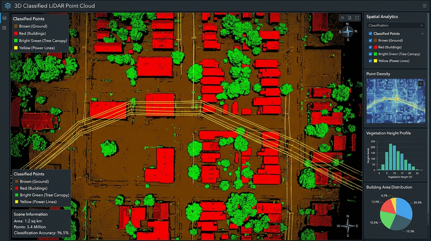
This guide demonstrates how to build a practical LiDAR point cloud classification Python laspy scikit-learn pipeline. We will read point-cloud data, explore noise reduction and voxel downsampling with Open3D, engineer local geometric features, train a Random Forest classifier, evaluate its predictions, and export the results into a standards-compliant LAS file.
The example targets four classes: ground, buildings, vegetation canopy, and power lines.
1. Environment Setup and Prerequisites
Python provides a flexible collection of open-source libraries for LiDAR processing and machine learning.
Required libraries
| Library | Purpose |
|---|---|
laspy |
Read, modify, and write LAS/LAZ point-cloud files |
numpy |
Efficient numerical operations on coordinates and features |
scikit-learn |
Train classifiers and evaluate predictions |
open3d |
Point-cloud downsampling, filtering, and visualization |
matplotlib |
Plot confusion matrices and diagnostic charts |
scipy |
Efficient nearest-neighbor searches using KD-trees |
Create a virtual environment and install the dependencies:
python -m venv lidar-envActivate it on Windows:
lidar-env\Scripts\activateOn Linux or macOS:
source lidar-env/bin/activateInstall the libraries, including an optional LAZ compression backend:
pip install "laspy[lazrs]" numpy scikit-learn open3d matplotlib scipylaspy supports LAS directly and uses optional backends such as lazrs to read and write compressed LAZ files. Review the laspy installation documentation if your dataset uses compression or requires a different backend.
You should also have a labeled training dataset containing representative examples of the classes you want to identify. Supervised machine learning cannot learn ground, buildings, vegetation, or power lines from geometry alone without reference labels.
2. Understanding LAS and LAZ Point-Cloud Data
LAS is a standardized format for exchanging LiDAR point-cloud data. LAZ stores the same type of information using lossless compression.
A point record may contain:
- X, Y, and Z coordinates.
- Laser-return intensity.
- Return number and number of returns.
- Classification and classification flags.
- GPS time, scan angle, and point source.
- RGB or near-infrared attributes, when available.
The LAS header stores metadata such as the point format, coordinate scales, offsets, bounds, and potentially coordinate reference system information.
One important distinction in laspy is that uppercase dimensions such as las.X, las.Y, and las.Z represent the underlying integer coordinates. The lowercase attributes las.x, las.y, and las.z expose coordinates with the header’s scale and offset applied.
For geometric calculations, use the scaled coordinates.
Standard classification codes
The example uses these ASPRS-compatible class codes:
| Target class | LAS classification code |
|---|---|
| Ground | 2 |
| Canopy | 5 — high vegetation |
| Building | 6 |
| Power line | 14 — wire conductor |
These codes follow the ASPRS LAS 1.4 specification.
The canopy class is represented by high vegetation in this simplified workflow, while power lines are represented by wire-conductor points. These semantic groupings are not interchangeable with arbitrary machine-learning label numbers. Always document your mapping when training and exporting classifications.
3. Step One: Read LAS and LAZ Files in Python
Begin by loading a labeled reference point cloud and a separate target point cloud. In a production workflow, the reference file should contain reliably labeled points from one or more representative scenes.
import laspy
import numpy as np

train_las = laspy.read("labeled_training.las")
target_las = laspy.read("target.las")

def extract_coordinates(las):
    return np.column_stack((
        las.x,
        las.y,
        las.z
    )).astype(np.float32)

train_xyz = extract_coordinates(train_las)
target_xyz = extract_coordinates(target_las)

train_intensity = np.asarray(
    train_las.intensity,
    dtype=np.float32
)

target_intensity = np.asarray(
    target_las.intensity,
    dtype=np.float32
)

train_labels = np.asarray(
    train_las.classification,
    dtype=np.uint8
)

print("Training points:", len(train_xyz))
print("Target points:", len(target_xyz))
print("LAS version:", target_las.header.version)
print("Point format:", target_las.header.point_format.id)
print("Available dimensions:",
      list(target_las.point_format.dimension_names))
The two input files serve different purposes. The labeled dataset supplies examples for learning the relationship between point-cloud features and object classes. The target dataset is the scene to classify.
Important: This example loads both files into memory. For large datasets, use the chunked-processing strategy described later rather than assuming every tile will fit into RAM.
4. Step Two: Noise Reduction and Voxel Downsampling with Open3D
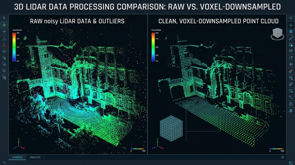
Raw LiDAR datasets can contain isolated returns, measurement noise, and uneven sampling density. Open3D provides statistical outlier removal and voxel-grid downsampling to help inspect and simplify point clouds.
Statistical outlier removal identifies points whose average neighbor distances are unusually large. Voxel downsampling groups nearby points into three-dimensional grid cells and represents each occupied cell with a representative point.
import open3d as o3d

def downsample_for_inspection(xyz, voxel_size=0.25):
    cloud = o3d.geometry.PointCloud()
    cloud.points = o3d.utility.Vector3dVector(
        xyz.astype(np.float64)
    )

    # Remove statistical outliers.
    filtered, _ = cloud.remove_statistical_outlier(
        nb_neighbors=20,
        std_ratio=2.0
    )

    # Reduce point density with a voxel grid.
    downsampled = filtered.voxel_down_sample(
        voxel_size=voxel_size
    )

    return downsampled

preview_cloud = downsample_for_inspection(
    target_xyz,
    voxel_size=0.25
)

print("Original points:", len(target_xyz))
print("Preview points:", len(preview_cloud.points))

o3d.visualization.draw_geometries([preview_cloud])
Here, voxel_size=0.25 uses a 25-centimeter voxel when the coordinates are expressed in meters. Select the voxel size according to point density, object dimensions, and the level of detail required.
A critical limitation applies: voxel downsampling changes the point representation, and statistical filtering may remove legitimate sparse returns. Thin power lines are particularly vulnerable to aggressive filtering.
Therefore, use this reduced cloud for inspection and exploratory analysis, not as a replacement for the original point records in the final classified output. The next steps calculate features from the original point geometry so every target point can receive a prediction.
For more detail, see the Open3D point-cloud API documentation.
5. Step Three: Geometric Feature Engineering
The success of machine-learning point-cloud classification depends heavily on feature quality. Raw coordinates alone rarely provide enough information to distinguish all object types reliably.
A flat roof, a ground surface, and a patch of vegetation can occupy similar elevations. Local geometric features describe how points are distributed around each return, helping the classifier distinguish surface shapes.
Understanding local covariance features
For each point, identify its nearest neighbors and compute a local covariance matrix. Its eigenvalues describe the dominant directions of spatial variation.
Let the ordered eigenvalues satisfy (\lambda_1 \geq \lambda_2 \geq \lambda_3 \geq 0).
Three commonly used features are:
- Linearity: ((\lambda_1-\lambda_2)/\lambda_1). High values indicate a dominant linear structure.
- Planarity: ((\lambda_2-\lambda_3)/\lambda_1). High values indicate a locally planar surface.
- Sphericity: (\lambda_3/\lambda_1). Higher values indicate a more isotropic, volumetric neighborhood.
Verticality is derived from the local surface normal, which corresponds to the eigenvector associated with the smallest eigenvalue. If (n_z) is the vertical component of that normal, define verticality as (1-|n_z|). This makes vertical surfaces score higher than horizontal surfaces.
We also calculate local roughness and relative height above a low neighborhood elevation percentile. These features help distinguish ground returns from elevated surfaces.
Calculate features using a KD-tree
The following implementation uses scipy.spatial.cKDTree for efficient nearest-neighbor queries and NumPy for covariance calculations.
from scipy.spatial import cKDTree

def compute_features(xyz, intensity, k=24):
    xyz = np.asarray(xyz, dtype=np.float32)
    intensity = np.asarray(intensity, dtype=np.float32)

    if len(xyz) < 3:
        raise ValueError(
            "At least three points are required."
        )

    k_eff = min(k + 1, len(xyz))

    tree = cKDTree(xyz)
    _, indices = tree.query(
        xyz,
        k=k_eff,
        workers=-1
    )

    # Exclude the nearest result, normally the point itself.
    neighbors = xyz[indices[:, 1:]]

    # Local covariance matrices.
    centered = neighbors - neighbors.mean(
        axis=1,
        keepdims=True
    )

    covariance = np.einsum(
        "nki,nkj->nij",
        centered,
        centered
    ) / neighbors.shape[1]

    eigenvalues, eigenvectors = np.linalg.eigh(
        covariance
    )

    l3 = np.maximum(eigenvalues[:, 0], 0)
    l2 = np.maximum(eigenvalues[:, 1], 0)
    l1 = np.maximum(eigenvalues[:, 2], 1e-12)

    linearity = (l1 - l2) / l1
    planarity = (l2 - l3) / l1
    sphericity = l3 / l1

    # Normal is the eigenvector of the smallest eigenvalue.
    normal_z = np.abs(eigenvectors[:, 2, 0])
    verticality = 1.0 - normal_z

    neighbor_z = neighbors[:, :, 2]
    relative_height = (
        xyz[:, 2]
        - np.quantile(neighbor_z, 0.10, axis=1)
    )

    roughness = np.sqrt(l3)

    # Approximate normalization for typical 16-bit intensity.
    intensity_norm = intensity / 65535.0

    return np.column_stack((
        intensity_norm,
        relative_height,
        linearity,
        planarity,
        sphericity,
        verticality,
        roughness
    )).astype(np.float32)
Each point now has seven features: normalized intensity, relative height, linearity, planarity, sphericity, verticality, and roughness.
The neighborhood parameter matters. A small neighborhood captures fine structures, while a larger neighborhood captures broader surface patterns. Test several values on representative data.
This implementation is suitable for manageable point-cloud tiles. Its neighbor-index arrays and covariance calculations can consume substantial memory when millions of points are processed simultaneously.
Also note that local features depend on point density and neighborhood composition. For robust transfer between datasets, keep feature definitions consistent and evaluate on geographically independent data.
6. Step Four: Train a Random Forest Classifier
A Random Forest combines many decision trees to predict a class from a feature vector. It works well as a baseline for LiDAR classification because it can capture nonlinear feature relationships and does not require feature standardization.
We will train the model to distinguish ground, canopy, buildings, and power lines.
Prepare the training data
from sklearn.ensemble import RandomForestClassifier
from sklearn.model_selection import train_test_split
from sklearn.metrics import (
    classification_report,
    ConfusionMatrixDisplay
)
import matplotlib.pyplot as plt

CLASS_CODES = {
    "ground": 2,
    "canopy": 5,
    "building": 6,
    "power_line": 14
}

class_codes = list(CLASS_CODES.values())
class_names = list(CLASS_CODES.keys())

X_all = compute_features(
    train_xyz,
    train_intensity,
    k=24
)

valid = np.isin(train_labels, class_codes)

X = X_all[valid]
y = train_labels[valid]

if len(y) == 0:
    raise ValueError(
        "No training points match the requested class codes."
    )

print("Training samples:", len(y))
print("Classes represented:", np.unique(y))
The reference file must contain actual labels for the requested classes. A model cannot learn four classes if some are missing from the training samples.
Fit the model and evaluate predictions
X_train, X_test, y_train, y_test = train_test_split(
    X,
    y,
    test_size=0.20,
    random_state=42,
    stratify=y
)

model = RandomForestClassifier(
    n_estimators=300,
    min_samples_leaf=2,
    class_weight="balanced_subsample",
    n_jobs=-1,
    random_state=42
)

model.fit(X_train, y_train)

y_pred = model.predict(X_test)

print(classification_report(
    y_test,
    y_pred,
    labels=class_codes,
    target_names=class_names,
    zero_division=0
))

ConfusionMatrixDisplay.from_predictions(
    y_test,
    y_pred,
    labels=class_codes,
    display_labels=class_names,
    cmap="Blues",
    xticks_rotation=45
)

plt.title("LiDAR Point Classification: Random Forest")
plt.tight_layout()
plt.savefig("lidar_confusion_matrix.png", dpi=200)
plt.show()
The classification report gives precision, recall, F1-score, and sample support for each class. The confusion matrix reveals which categories are being confused. For example, a model may mistake vegetation for ground or classify building edges as power lines.
The random train-test split above is intended as a basic demonstration. Neighboring LiDAR points are spatially correlated, so randomly splitting points from the same scene can overestimate real-world accuracy. For a credible assessment, hold out an entire spatial block, survey area, or separate labeled tile whenever possible.
7. Step Five: Classify the Target Point Cloud
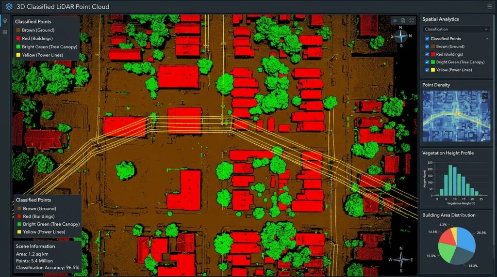
After evaluating the model, calculate the same features for the target file and generate predictions.
target_features = compute_features(
    target_xyz,
    target_intensity,
    k=24
)

target_predictions = model.predict(
    target_features
)

print("Predicted points:", len(target_predictions))
print(
    "Predicted LAS classes:",
    np.unique(target_predictions)
)
The model uses the same feature order and parameters as during training. Changing the neighborhood size, intensity transformation, or feature definitions between training and prediction can undermine the results.
Predictions may still be imperfect. Thin wires, tree branches, building edges, and low-density areas often require careful feature tuning or additional return attributes.
8. Step Six: Export Classified Points to LAS
A reliable export should preserve the original file’s coordinate information and metadata wherever possible.
Rather than constructing a new file from XYZ arrays, update the classification dimension on the loaded target object. This preserves its original point records and existing header information, including coordinate scales, offsets, point format, and available CRS metadata.
# Assign predicted ASPRS-compatible class codes.
target_las.classification = (
    target_predictions.astype(np.uint8)
)

# Save as an uncompressed LAS file.
target_las.write("classified_target.las")

print("Saved classified_target.las")
To write compressed LAZ output instead, change the filename:
target_las.write("classified_target.laz")The installed LAZ backend must support the data being written. With the optional lazrs dependency installed, typical LAS/LAZ workflows are supported, subject to backend limitations.
Because the example retains all original point records and coordinates, it does not need to reconstruct the LAS header from scratch. This is safer than creating a new default header, which may lose the source coordinate scales, offsets, CRS information, or other metadata.
If you create an entirely new point cloud from arrays, you must explicitly choose a compatible LAS version and point format, set appropriate coordinate scales and offsets, preserve or add CRS metadata, and populate the supported point dimensions correctly.
Extract ground returns
The classified file can now be used to isolate ground points for digital terrain modeling or additional surface analysis.
ground_mask = (
    target_las.classification
    == CLASS_CODES["ground"]
)

ground_points = target_las.points[ground_mask]

ground_las = laspy.LasData(
    target_las.header.copy()
)

ground_las.points = ground_points
ground_las.write("ground_returns.las")
The output contains only the points classified as ground, with the source header copied as a starting point. Validate the resulting file in a LAS-aware viewer or with laspy before downstream use.
9. Performance Optimization for Large Point Clouds
Processing a multi-gigabyte LiDAR tile requires a different strategy from processing a small sample. Loading all coordinates, neighbors, covariance matrices, and features simultaneously can exhaust available memory.
Use chunked LAS/LAZ reading
laspy.open() supports reading point records in chunks. This is useful for inspection, filtering, conversion, and larger workflows.
import laspy

with laspy.open("large_tile.laz") as reader:
    print("Total points:", reader.header.point_count)

    for points in reader.chunk_iterator(500_000):
        xyz = np.column_stack((
            points.x,
            points.y,
            points.z
        ))

        intensity = points.intensity

        # Process this chunk or write its records
        # to an appropriate intermediate dataset.
This example shows memory-conscious reading, not a complete neighborhood-aware classifier. A chunk_iterator divides the file’s record sequence, which is not guaranteed to correspond to spatially compact blocks. Points close to the boundary of two chunks may therefore be neighbors even when they appear in different batches.
For geometric feature extraction, use spatial tiles with overlapping buffer zones. Compute features using the core tile plus its surrounding halo, predict classes for the core points, and write each core exactly once. Buffer width and neighborhood size must be chosen to capture sufficient spatial context.
A scalable production pipeline can follow this pattern:
- Partition the point cloud into spatial tiles.
- Read each tile together with a neighborhood buffer.
- Compute local features using the buffered points.
- Predict classes for the tile’s core points only.
- Write predictions and retain the original point dimensions.
- Merge or index the completed outputs where appropriate.
For extremely large datasets, consider spatially indexed formats and tiling tools rather than assuming a single Python array can represent the entire scene.
Additional optimization techniques
Reduce feature-array memory. Use float32 for coordinates and feature matrices where its precision is adequate. Process smaller tiles to limit the size of temporary neighbor arrays.
Tune the neighborhood size. Increasing the number of neighbors increases computational cost and may blur boundaries. Start with a moderate value such as 24, then benchmark alternative settings against labeled validation data.
Avoid indiscriminate denoising. Statistical filters can remove legitimate low-density returns, especially wires and fine vegetation. Preserve original records and evaluate filtering choices by class.
Use multiple informative attributes. Where available, include return number, number of returns, RGB, scan angle, and additional sensor attributes. Normalize and document each feature consistently.
Use class-aware evaluation. Overall accuracy can hide poor power-line detection when power-line returns constitute a tiny fraction of the dataset. Compare per-class precision, recall, and F1-score, and investigate errors using a 3D viewer.
Parallelize carefully. Random Forest training can use multiple CPU cores through n_jobs=-1. However, parallel jobs and large feature matrices can increase peak memory consumption. Benchmark the complete workflow rather than optimizing a single isolated operation.
10. Common Pitfalls and Troubleshooting
| Problem | Likely cause | Recommended action |
|---|---|---|
| Unable to open LAZ files | Missing or incompatible compression backend | Install laspy[lazrs] and verify the backend |
| Poor ground classification | Weak height or local surface features | Tune neighborhood size and add suitable elevation context |
| Power lines classified as vegetation | Sparse returns and class imbalance | Add linearity and return attributes; increase representative wire samples |
| Excellent test score but poor results on new areas | Spatial leakage between training and test points | Validate on separate spatial blocks or tiles |
| Coordinates appear shifted | Scales, offsets, or CRS interpretation errors | Inspect the LAS header and scaled coordinates |
| Excessive memory usage | Large intermediate arrays and global neighbor searches | Use buffered spatial tiles and smaller feature batches |
A further limitation is that covariance features describe local geometry, not object identity. A narrow branch, cable, and other linear structure may share similar feature values. Better results may require more representative training data, additional sensor attributes, contextual rules, or a specialized point-cloud segmentation model.
11. SEO Interlinking and Further Reading
Build topical relevance by connecting this tutorial to related GIS developer resources on your website.
Suggested internal links:
- Python GeoPandas automation guide — for integrating classified spatial outputs into automated geoprocessing workflows.
- Spatial machine learning guide — for validation strategies, feature engineering, and model selection.
- Point pattern analysis guide — for analyzing the spatial distributions of extracted features and classified point populations.
Replace these suggested paths with the live URLs on your website.
Recommended external references:
- laspy documentation — LAS/LAZ reading, writing, and point-record manipulation.
- Open3D documentation — point-cloud filtering, downsampling, and geometric operations.
- Scikit-Learn RandomForestClassifier — model parameters and prediction behavior.
- ASPRS LAS 1.4 specification — standard point-class definitions and LAS record structure.
Conclusion
Programmatic LiDAR point cloud classification in Python provides a repeatable alternative to manually classifying every point in desktop GIS software. By combining laspy for LAS/LAZ data handling, Open3D for exploratory point-cloud operations, NumPy and KD-trees for geometric feature engineering, and Scikit-Learn for Random Forest classification, spatial analysts can develop automated 3D processing pipelines.
The workflow covered in this guide reads source point clouds, derives local geometric features, trains and evaluates a supervised classifier, predicts ground, canopy, building, and power-line classes, and exports the results while preserving source metadata.
For production deployment, prioritize representative reference labels, spatially independent validation, consistent feature calculations, class-aware evaluation, and memory-conscious spatial tiling. These measures are especially important when working with sparse structures, large urban datasets, or multi-gigabyte point-cloud tiles.
Code repository reference: Organize the workflow into a reusable Python project containing feature extraction, model training, validation, prediction, and LAS export modules. Include a requirements.txt file, a README explaining the expected input schemas and ASPRS class mappings, and a small sample dataset or synthetic test case. Store trained models and validation metrics alongside documented parameter settings so that subsequent classification runs remain reproducible.