Table of Contents

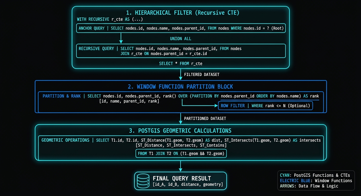
Spatial Window Functions and Recursive CTEs in PostGIS

Introduction

Complex spatial analysis in PostgreSQL rarely requires abandoning SQL for procedural code. By combining PostgreSQL’s analytical SQL features with PostGIS geometry functions, it is possible to build sophisticated workflows for trajectory analysis, spatial hierarchies, network-like traversals, and sequential geographic processes entirely inside the database.

Two SQL capabilities are particularly powerful:

Window functions such as LAG(), LEAD(), ROW_NUMBER(), and SUM() OVER() for analyzing ordered spatial observations.
Common Table Expressions (CTEs), including recursive CTEs, for breaking complicated spatial workflows into logical stages and traversing parent-child relationships.

For example, a GPS trajectory can be represented as an ordered sequence of points:

P1 → P2 → P3 → P4 → P5

A window query can compare each point with the preceding or following point without performing an explicit self-join. PostGIS then calculates the spatial relationship between those points:

ST_Distance(previous_point, current_point)

Similarly, administrative boundaries or nested watersheds can be represented as hierarchical relationships:

Country
└── Region
    └── District
        └── Subdivision

A recursive CTE can traverse this hierarchy until the desired spatial level is reached.

The combination is especially useful because PostGIS handles spatial computation while PostgreSQL handles relational ordering, partitioning, and recursion.

1. Spatial Window Functions Recursive CTEs PostGIS for Movement & Trajectory Analysis

1.1 Understanding the spatial window

A normal SQL query might calculate the distance between two known geometries:

SELECT
    ST_Distance(a.geom, b.geom)
FROM points a
JOIN points b
    ON a.id = b.id;

The difficulty appears when the relationship is sequential.

Suppose a GPS table contains:

track_id | timestamp | geom
---------+-----------+----------------
101      | 08:00     | Point 1
101      | 08:01     | Point 2
101      | 08:02     | Point 3
101      | 08:03     | Point 4

We want:

Point 1 → Point 2
Point 2 → Point 3
Point 3 → Point 4

Rather than repeatedly joining the table against itself, LAG() can expose the previous geometry.

LAG(geom) OVER (
    PARTITION BY track_id
    ORDER BY recorded_at
)

This produces a virtual previous-point column for every observation.

1.2 Calculating step-by-step distance

Assume a table called gps_points:

CREATE TABLE gps_points (
    id          BIGSERIAL PRIMARY KEY,
    track_id    INTEGER NOT NULL,
    recorded_at TIMESTAMPTZ NOT NULL,
    geom        geometry(Point, 4326) NOT NULL
);

The first analytical step is retrieving the previous point.

SELECT
    id,
    track_id,
    recorded_at,
    geom,

    LAG(geom) OVER (
        PARTITION BY track_id
        ORDER BY recorded_at
    ) AS previous_geom

FROM gps_points;

The result conceptually becomes:

Point	Previous Point
P1	NULL
P2	P1
P3	P2
P4	P3

We can then calculate the distance.

For geographic coordinates, ST_Distance should generally be used carefully because geometry coordinates in EPSG:4326 are expressed in degrees.

One robust approach is transforming the points into an appropriate projected coordinate system.

For example:

WITH ordered_points AS (
    SELECT
        id,
        track_id,
        recorded_at,
        geom,

        LAG(geom) OVER (
            PARTITION BY track_id
            ORDER BY recorded_at
        ) AS previous_geom

    FROM gps_points
)

SELECT
    id,
    track_id,
    recorded_at,

    ST_Distance(
        ST_Transform(previous_geom, 32737),
        ST_Transform(geom, 32737)
    ) AS step_distance_m

FROM ordered_points
WHERE previous_geom IS NOT NULL;

Here, 32737 represents WGS 84 / UTM zone 37S, which is appropriate for much of Kenya.

For a production system covering a large geographic region, the projected CRS should instead be selected according to the actual spatial extent of the data.

1.3 Using geography for geodesic distance

Another option is to cast geometries to geography.

ST_Distance(
    previous_geom::geography,
    geom::geography
)

This calculates distance on the Earth’s surface in meters.

A complete query becomes:

WITH ordered_points AS (
    SELECT
        id,
        track_id,
        recorded_at,
        geom,

        LAG(geom) OVER (
            PARTITION BY track_id
            ORDER BY recorded_at
        ) AS previous_geom

    FROM gps_points
)

SELECT
    id,
    track_id,
    recorded_at,

    ST_Distance(
        previous_geom::geography,
        geom::geography
    ) AS step_distance_m

FROM ordered_points
WHERE previous_geom IS NOT NULL;

This approach is convenient for GPS data stored in WGS 84.

2. Calculating Movement Speed

Once step distance has been calculated, velocity can be derived from the elapsed time between observations.

Use another LAG() expression:

LAG(recorded_at) OVER (
    PARTITION BY track_id
    ORDER BY recorded_at
)

A production-oriented query can calculate both distance and elapsed time.

WITH ordered_points AS (
    SELECT
        id,
        track_id,
        recorded_at,
        geom,

        LAG(geom) OVER (
            PARTITION BY track_id
            ORDER BY recorded_at
        ) AS previous_geom,

        LAG(recorded_at) OVER (
            PARTITION BY track_id
            ORDER BY recorded_at
        ) AS previous_time

    FROM gps_points
),

movement AS (
    SELECT
        id,
        track_id,
        recorded_at,

        ST_Distance(
            previous_geom::geography,
            geom::geography
        ) AS distance_m,

        EXTRACT(
            EPOCH FROM (
                recorded_at - previous_time
            )
        ) AS elapsed_seconds

    FROM ordered_points
    WHERE previous_geom IS NOT NULL
      AND previous_time IS NOT NULL
)

SELECT
    id,
    track_id,
    recorded_at,
    distance_m,
    elapsed_seconds,

    CASE
        WHEN elapsed_seconds > 0
        THEN distance_m / elapsed_seconds
        ELSE NULL
    END AS speed_mps,

    CASE
        WHEN elapsed_seconds > 0
        THEN (distance_m / elapsed_seconds) * 3.6
        ELSE NULL
    END AS speed_kmh

FROM movement;

The important design principle is to separate the workflow into CTE stages:

Raw GPS points
      ↓
Ordered points
      ↓
Previous point/time
      ↓
Distance + elapsed time
      ↓
Speed

This makes the SQL much easier to test and extend.

3. Calculating Heading Angles

Distance alone does not describe movement direction.

For trajectory analysis, we may also need the heading or bearing between consecutive GPS points.

PostGIS provides:

ST_Azimuth()

For geometry coordinates, the function returns the angle in radians measured clockwise from north.

We can convert the result to degrees:

DEGREES(
    ST_Azimuth(previous_geom, geom)
)

A complete trajectory query is:

WITH ordered_points AS (
    SELECT
        id,
        track_id,
        recorded_at,
        geom,

        LAG(geom) OVER (
            PARTITION BY track_id
            ORDER BY recorded_at
        ) AS previous_geom

    FROM gps_points
)

SELECT
    id,
    track_id,
    recorded_at,

    ST_Distance(
        previous_geom::geography,
        geom::geography
    ) AS distance_m,

    CASE
        WHEN previous_geom IS NOT NULL
        THEN DEGREES(
            ST_Azimuth(
                previous_geom::geography,
                geom::geography
            )
        )
        ELSE NULL
    END AS heading_degrees

FROM ordered_points;

A heading of approximately:

0°   = North
90°  = East
180° = South
270° = West

The result can therefore support analyses such as:

vehicle movement direction,
pedestrian trajectories,
animal tracking,
maritime movement,
delivery routes,
mobility studies.

4. Comparing Consecutive Headings

Window functions become even more useful when several sequential calculations are combined.

Suppose we want to detect sharp turns.

First calculate each segment’s heading:

WITH ordered_points AS (
    SELECT
        id,
        track_id,
        recorded_at,
        geom,

        LAG(geom) OVER (
            PARTITION BY track_id
            ORDER BY recorded_at
        ) AS previous_geom

    FROM gps_points
),

headings AS (
    SELECT
        id,
        track_id,
        recorded_at,

        DEGREES(
            ST_Azimuth(
                previous_geom::geography,
                geom::geography
            )
        ) AS heading

    FROM ordered_points
    WHERE previous_geom IS NOT NULL
)

SELECT
    *,
    LAG(heading) OVER (
        PARTITION BY track_id
        ORDER BY recorded_at
    ) AS previous_heading

FROM headings;

A subsequent calculation can determine heading change.

However, angles wrap around at 360°.

For example:

Previous = 350°
Current  = 10°

The naïve difference is:

10 - 350 = -340°

But the actual turn is only:

+20°

A normalized angular difference can be calculated as:

((current_heading - previous_heading + 540) % 360) - 180

This produces a range from:

-180° to +180°

A trajectory system can then classify large angular changes as potential turns.

5. Using LEAD() for Forward-Looking Analysis

LAG() looks backward.

LEAD() looks forward.

For example:

LEAD(geom) OVER (
    PARTITION BY track_id
    ORDER BY recorded_at
)

can identify the next GPS point.

This is useful when the analytical question is:

What happens after this observation?

For example:

SELECT
    id,
    track_id,
    recorded_at,
    geom,

    LEAD(geom) OVER (
        PARTITION BY track_id
        ORDER BY recorded_at
    ) AS next_geom

FROM gps_points;

You can then calculate the distance from the current point to the next point.

This is particularly useful for generating segment-level representations:

Point 1 ───── Point 2
Point 2 ───── Point 3
Point 3 ───── Point 4

6. Creating Trajectory Segments

A useful production pattern is converting consecutive GPS points into line segments.

WITH ordered_points AS (
    SELECT
        id,
        track_id,
        recorded_at,
        geom,

        LEAD(geom) OVER (
            PARTITION BY track_id
            ORDER BY recorded_at
        ) AS next_geom

    FROM gps_points
)

SELECT
    id,
    track_id,
    recorded_at,

    ST_MakeLine(
        geom,
        next_geom
    ) AS segment_geom

FROM ordered_points

WHERE next_geom IS NOT NULL;

This transforms point observations into movement segments.

The resulting table can be used for:

route visualization,
segment speed analysis,
road matching,
trajectory simplification,
movement heatmaps.

7. Recursive CTEs for Hierarchical Spatial Boundaries

Window functions are excellent for sequential analysis, but they do not solve hierarchical traversal.

Consider a database containing nested spatial units:

National Boundary
│
├── County
│   ├── Subcounty
│   │   ├── Ward
│   │   └── Ward
│   └── Subcounty
│
└── County

The hierarchy can be represented relationally:

CREATE TABLE spatial_units (
    id          BIGSERIAL PRIMARY KEY,
    name        TEXT NOT NULL,
    parent_id   BIGINT REFERENCES spatial_units(id),
    unit_type   TEXT NOT NULL,
    geom        geometry(MultiPolygon, 4326)
);

The important relationship is:

parent_id → id

This means the spatial hierarchy is not necessarily determined by geometry alone. It is an explicit relational tree.

8. Basic Recursive CTE

Suppose we want to retrieve an entire hierarchy starting from a particular root.

WITH RECURSIVE hierarchy AS (

    -- Anchor member: start with the root
    SELECT
        id,
        name,
        parent_id,
        unit_type,
        geom,
        0 AS depth

    FROM spatial_units

    WHERE id = 1

    UNION ALL

    -- Recursive member: find children
    SELECT
        child.id,
        child.name,
        child.parent_id,
        child.unit_type,
        child.geom,
        parent.depth + 1

    FROM spatial_units AS child

    JOIN hierarchy AS parent
        ON child.parent_id = parent.id
)

SELECT *
FROM hierarchy
ORDER BY depth, id;

The recursive process is:

Root
 ↓
Children
 ↓
Grandchildren
 ↓
Great-grandchildren
 ↓
...

The depth column records how far each record is from the root.

9. Building a Hierarchical Spatial Path

A powerful extension is maintaining the complete ancestry path.

WITH RECURSIVE hierarchy AS (

    SELECT
        id,
        name,
        parent_id,
        unit_type,
        geom,

        0 AS depth,

        ARRAY[id] AS path

    FROM spatial_units

    WHERE id = 1

    UNION ALL

    SELECT
        child.id,
        child.name,
        child.parent_id,
        child.unit_type,
        child.geom,

        parent.depth + 1,

        parent.path || child.id

    FROM spatial_units AS child

    JOIN hierarchy AS parent
        ON child.parent_id = parent.id
)

SELECT
    id,
    name,
    unit_type,
    depth,
    path

FROM hierarchy

ORDER BY path;

A path might look like:

{1}
{1,4}
{1,4,12}
{1,4,12,27}

This makes the hierarchy explicitly queryable.

10. Recursive Spatial Processing

The recursive CTE becomes particularly interesting when geometry itself participates in the analysis.

For example, suppose subdivisions are stored as children and we want to determine their relationship with the parent geometry.

WITH RECURSIVE hierarchy AS (

    SELECT
        id,
        name,
        parent_id,
        unit_type,
        geom,
        0 AS depth

    FROM spatial_units

    WHERE parent_id IS NULL

    UNION ALL

    SELECT
        child.id,
        child.name,
        child.parent_id,
        child.unit_type,
        child.geom,
        parent.depth + 1

    FROM spatial_units child

    JOIN hierarchy parent
        ON child.parent_id = parent.id

    WHERE ST_Within(
        child.geom,
        parent.geom
    )
)

SELECT
    id,
    name,
    unit_type,
    depth

FROM hierarchy;

The important distinction is that recursion determines which records are traversed, while PostGIS functions can validate or analyze their spatial relationships.

11. Example: Nested Watersheds

Consider a watershed database:

Large Catchment
   ↓
Sub-Catchment
   ↓
Micro-Catchment

The table could contain:

CREATE TABLE watersheds (
    watershed_id BIGSERIAL PRIMARY KEY,
    parent_id    BIGINT,
    name         TEXT,
    geom         geometry(MultiPolygon, 4326)
);

A recursive query can identify all descendants of a selected watershed:

WITH RECURSIVE watershed_tree AS (

    SELECT
        watershed_id,
        parent_id,
        name,
        geom,
        0 AS level

    FROM watersheds

    WHERE watershed_id = 100

    UNION ALL

    SELECT
        w.watershed_id,
        w.parent_id,
        w.name,
        w.geom,
        wt.level + 1

    FROM watersheds w

    JOIN watershed_tree wt
        ON w.parent_id = wt.watershed_id
)

SELECT
    watershed_id,
    name,
    level,
    ST_Area(geom::geography) AS area_m2

FROM watershed_tree

ORDER BY level, watershed_id;

Now the recursion produces the hierarchy while PostGIS calculates the physical area of every spatial unit.

12. Combining Recursive CTEs With Spatial Aggregation

The output of a recursive query can be used as a spatial analytical dataset.

For example:

WITH RECURSIVE watershed_tree AS (

    SELECT
        watershed_id,
        parent_id,
        name,
        geom,
        0 AS level

    FROM watersheds

    WHERE watershed_id = 100

    UNION ALL

    SELECT
        child.watershed_id,
        child.parent_id,
        child.name,
        child.geom,
        parent.level + 1

    FROM watersheds child

    JOIN watershed_tree parent
        ON child.parent_id = parent.watershed_id
)

SELECT
    level,

    COUNT(*) AS watershed_count,

    SUM(
        ST_Area(geom::geography)
    ) AS total_area_m2

FROM watershed_tree

GROUP BY level

ORDER BY level;

This creates a hierarchical summary:

Level	Meaning
0	Root watershed
1	Direct subdivisions
2	Nested subdivisions
3	Deeper subdivisions

13. Hierarchical Spatial Queries With Containment

Not every spatial hierarchy has an explicit parent_id.

Sometimes the hierarchy must be derived from geometry.

For example, one layer may contain administrative boundaries at different levels:

County
Subcounty
Ward

A spatial relationship can establish the parent-child relationship:

ST_Contains(parent.geom, child.geom)

However, blindly using this inside a recursive query can become computationally expensive.

A better architecture is usually to materialize or persist the discovered parent relationship:

child_id | parent_id
---------+----------
10       | 2
11       | 2
12       | 5

Then recursion operates on the indexed relational relationship.

This separates two expensive problems:

Spatial containment
        ↓
Parent-child relationship
        ↓
Recursive hierarchy traversal

That design is generally easier to maintain and optimize.

14. Combining Window Functions and Recursive CTEs

The two techniques do not have to be isolated.

A sophisticated spatial workflow can use:

Recursive CTE
      ↓
Generate hierarchical subset
      ↓
Window function
      ↓
Analyze observations within each spatial unit
      ↓
PostGIS geometry calculations

For example, suppose GPS observations belong to nested operational zones.

A recursive CTE can retrieve all zones beneath a selected parent, after which a window function can analyze movement observations within each zone.

Conceptually:

WITH RECURSIVE zones AS (

    SELECT
        id,
        parent_id,
        name,
        0 AS depth

    FROM operational_zones

    WHERE id = 100

    UNION ALL

    SELECT
        child.id,
        child.parent_id,
        child.name,
        parent.depth + 1

    FROM operational_zones child

    JOIN zones parent
        ON child.parent_id = parent.id
),

zone_points AS (

    SELECT
        p.id,
        p.track_id,
        p.recorded_at,
        z.id AS zone_id,
        p.geom

    FROM gps_points p

    JOIN zones z
        ON ST_Within(p.geom, z.geom)
),

ordered_points AS (

    SELECT
        *,
        LAG(geom) OVER (
            PARTITION BY track_id, zone_id
            ORDER BY recorded_at
        ) AS previous_geom

    FROM zone_points
)

SELECT
    id,
    track_id,
    zone_id,
    recorded_at,

    ST_Distance(
        previous_geom::geography,
        geom::geography
    ) AS distance_m

FROM ordered_points

WHERE previous_geom IS NOT NULL;

This illustrates the larger principle:

CTEs define analytical stages; window functions define sequence; PostGIS defines spatial relationships.

15. Performance Considerations

Spatial window queries can become expensive when millions of observations are involved.

Performance should therefore be designed into the schema and query architecture rather than added afterward.

15.1 Spatial indexes

A GiST index should normally be created on geometry columns used in spatial filtering.

CREATE INDEX idx_gps_points_geom
ON gps_points
USING GIST (geom);

For hierarchy tables:

CREATE INDEX idx_spatial_units_geom
ON spatial_units
USING GIST (geom);

These indexes are particularly important for predicates such as:

ST_Within()
ST_Intersects()
ST_Contains()
ST_DWithin()

15.2 Index the recursive relationship

A recursive hierarchy frequently joins through:

child.parent_id = parent.id

Therefore:

CREATE INDEX idx_spatial_units_parent
ON spatial_units(parent_id);

This is often more important to recursive performance than the spatial index itself.

The database is performing a relational traversal:

parent_id → child records

so PostgreSQL needs an efficient way to find those children.

16. Indexing Window-Function Ordering

Window functions such as:

LAG(geom) OVER (
    PARTITION BY track_id
    ORDER BY recorded_at
)

require PostgreSQL to establish ordering within each track.

A composite index can help:

CREATE INDEX idx_gps_track_time
ON gps_points (
    track_id,
    recorded_at
);

This is particularly appropriate when the table is frequently queried by trajectory.

The index corresponds directly to the analytical structure:

track_id
   ↓
recorded_at
   ↓
sequential observations

17. Avoid Repeated Coordinate Transformations

A common performance mistake is repeatedly transforming the same geometry:

ST_Transform(geom, 32737)

inside multiple expressions.

For large datasets, consider storing an appropriate projected representation when justified by the application’s spatial requirements.

For example:

ALTER TABLE gps_points
ADD COLUMN geom_utm geometry(Point, 32737);

Then populate it:

UPDATE gps_points
SET geom_utm = ST_Transform(geom, 32737);

Create an index if spatial queries will use the projected geometry:

CREATE INDEX idx_gps_points_geom_utm
ON gps_points
USING GIST (geom_utm);

This should be evaluated carefully because maintaining duplicate geometry columns introduces storage and data-maintenance costs.

18. Be Careful With CTE Materialization

CTEs are logical query-building tools, but their execution behavior matters.

For expensive workflows, inspect the execution plan:

EXPLAIN (ANALYZE, BUFFERS)
WITH ordered_points AS (
    ...
)
SELECT ...

Modern PostgreSQL can inline suitable CTEs, while explicit materialization can be requested when appropriate:

WITH ordered_points AS MATERIALIZED (
    ...
)

or:

WITH ordered_points AS NOT MATERIALIZED (
    ...
)

Materialization can be useful when the intermediate result is expensive to generate but reused multiple times.

It can also hurt performance when it forces unnecessary storage and prevents useful optimization.

Therefore, do not assume that a CTE is automatically a performance optimization.

Treat it primarily as a query-organization mechanism and verify performance with EXPLAIN ANALYZE.

19. Partitioning Window Queries Correctly

The following query:

LAG(geom) OVER (
    ORDER BY recorded_at
)

would compare observations across every track.

That is usually incorrect.

Instead:

LAG(geom) OVER (
    PARTITION BY track_id
    ORDER BY recorded_at
)

ensures that the previous point belongs to the same trajectory.

This distinction is critical.

Without PARTITION BY:

Vehicle A → Vehicle B

could accidentally become a valid “movement segment.”

With partitioning:

Vehicle A:
P1 → P2 → P3

Vehicle B:
P1 → P2 → P3

each trajectory remains independent.

20. Validate Temporal Ordering

GPS data can contain duplicate or inconsistent timestamps.

This:

ORDER BY recorded_at

may therefore produce nondeterministic ordering when two observations have identical timestamps.

A safer pattern is:

ORDER BY recorded_at, id

For example:

LAG(geom) OVER (
    PARTITION BY track_id
    ORDER BY recorded_at, id
)

The unique id acts as a deterministic tie-breaker.

For production trajectory processing, this small detail can prevent subtle analytical errors.

21. Recursive CTE Safety

Recursive queries should always have a clearly defined termination condition.

In a properly modeled tree, recursion naturally stops when no additional children exist.

However, malformed data can contain cycles:

A → B → C → A

A defensive implementation can maintain a path and prevent revisiting nodes.

WITH RECURSIVE hierarchy AS (

    SELECT
        id,
        parent_id,
        name,
        ARRAY[id] AS path

    FROM spatial_units

    WHERE id = 1

    UNION ALL

    SELECT
        child.id,
        child.parent_id,
        child.name,
        parent.path || child.id

    FROM spatial_units child

    JOIN hierarchy parent
        ON child.parent_id = parent.id

    WHERE NOT child.id = ANY(parent.path)
)

SELECT *
FROM hierarchy;

The condition:

NOT child.id = ANY(parent.path)

prevents a node already encountered in the current path from being traversed again.

This is especially important when hierarchical data originates from multiple external systems.

Summary

Spatial Window Functions Recursive CTEs PostGIS combine three powerful capabilities:

PostgreSQL Window Functions
        +
Recursive CTEs
        +
PostGIS Spatial Functions

Window functions are particularly effective for sequential trajectory analysis. LAG() and LEAD() expose neighboring observations without cumbersome self-joins, allowing PostGIS to calculate:

step distances,
elapsed time,
speed,
heading,
turning angles,
trajectory segments.

Recursive CTEs solve a different class of problems: hierarchical spatial queries. They can traverse nested administrative units, watersheds, property subdivisions, organizational spatial zones, and other parent-child structures.

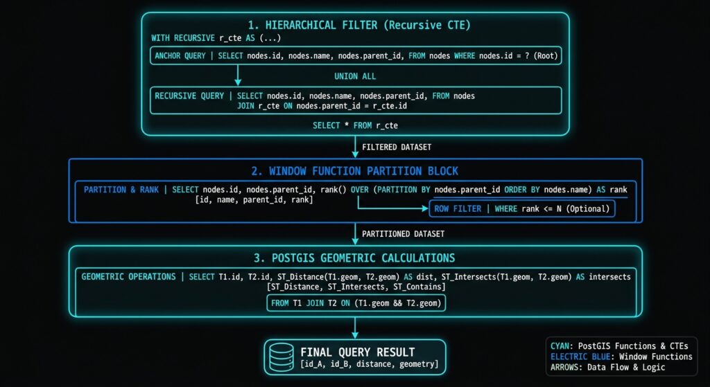
The strongest production architecture combines them:

Raw spatial data
      │
      ▼
Recursive CTE
      │
      ├── Identify spatial hierarchy
      │
      ▼
Filtered spatial dataset
      │
      ▼
Window functions
      │
      ├── LAG()
      ├── LEAD()
      ├── PARTITION BY
      └── ORDER BY
      │
      ▼
PostGIS calculations
      │
      ├── ST_Distance()
      ├── ST_Azimuth()
      ├── ST_Within()
      ├── ST_Contains()
      └── ST_Intersects()
      │
      ▼
Analytical result

For production systems, the key performance principles are equally important: GiST indexes for spatial predicates, B-tree indexes for hierarchical and temporal relationships, deterministic ordering for window functions, appropriate CRS handling, cycle protection for recursive queries, and EXPLAIN (ANALYZE, BUFFERS) for validation.

The result is a database-centric spatial processing architecture capable of handling sophisticated movement, hierarchy, and spatial relationship analysis without moving large datasets into external Python or GIS processing environments.