Extracting Building Footprints from Aerial Imagery Using OpenCV and Python

1. Introduction

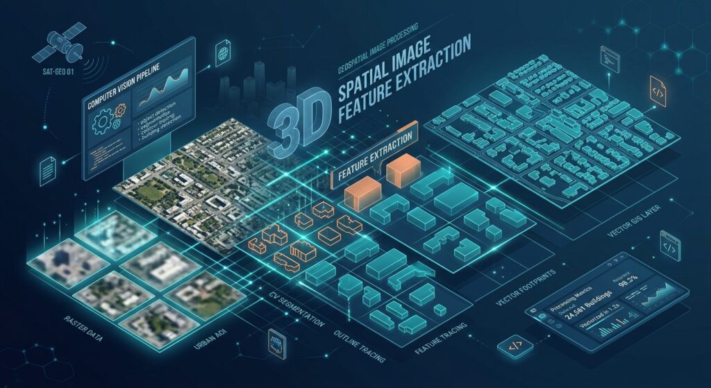
Mastering the fundamentals of extracting building footprints OpenCV Python offers a practical way to automate part of the building-mapping workflow before investing in deep learning models. Extracting building footprints with OpenCV and Python GIS tools offers a practical way to automate part of the building-mapping workflow before investing in deep learning models. High-resolution orthophotos contain visible roof edges, color variations, shadows, and geometric patterns that traditional computer vision techniques can use to identify candidate building outlines.

Digitizing thousands of roofs manually is time-consuming, especially when updating cadastral maps, preparing urban land-use inventories, or mapping rapidly expanding settlements. OpenCV provides image-processing algorithms for thresholding, edge detection, morphological operations, and contour extraction. Rasterio preserves the geospatial information stored in aerial imagery, while Shapely and GeoPandas convert detected contours into usable GIS vector features.

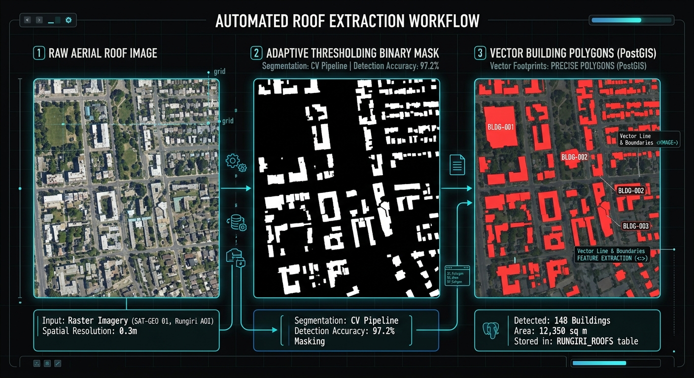
The workflow in this tutorial follows five stages:

This is a classical computer vision approach, not a trained building-recognition model. It works best on relatively clear imagery with distinguishable roofs. Trees, roads, parking lots, and shadows can also generate contours, so the result should be treated as a candidate building layer that requires validation.

2. Environment setup

Install the Python libraries

Create a Python environment and install the required packages:

python -m venv building_env

Activate the environment.

On Windows:

building_env\Scripts\activate

On Linux:

source building_env/bin/activate

Install the dependencies:

python -m pip install opencv-python rasterio shapely geopandas numpy

These libraries serve different purposes:

You will also need a georeferenced orthophoto, preferably a three-band RGB GeoTIFF with a valid coordinate reference system (CRS).

Important assumption: The following implementation expects the first three raster bands to represent red, green, and blue. Check the imagery’s band descriptions before processing because some products use different band orders or include additional bands.

3. Step 1 — Read the GeoTIFF and preserve spatial metadata

An ordinary image contains pixel values. A georeferenced raster additionally relates those pixels to real-world coordinates.

Rasterio exposes the raster’s CRS, bounds, dimensions, and affine transformation. The affine transformation is essential because OpenCV detects features using image coordinates, whereas a GIS polygon must use map coordinates.

Start by loading the first three bands and inspecting the metadata.

import rasterioimport numpy as npfrom pathlib import Path# Input orthophoto and output locations.INPUT_TIF = Path("aerial_orthophoto.tif")OUTPUT_GPKG = Path("building_footprints.gpkg")# Read the image and retain its geospatial metadata.with rasterio.open(INPUT_TIF) as src:    if src.count < 3:        raise ValueError("The input raster must contain at least 3 bands.")    if src.crs is None:        raise ValueError(            "The raster has no CRS. Define its correct CRS before processing."        )    # Read the first three bands as RGB candidates.    rgb_raw = src.read([1, 2, 3], out_dtype="float32")    # Rasterio returns (bands, rows, columns).    # Convert to the (rows, columns, channels) shape used by OpenCV.    rgb_raw = np.moveaxis(rgb_raw, 0, -1)    # Capture valid-data pixels to avoid processing nodata areas.    valid_mask = src.dataset_mask() > 0    # Save the spatial metadata for later use.    raster_transform = src.transform    raster_crs = src.crs    raster_bounds = src.bounds    print("Raster dimensions:", src.width, "x", src.height)    print("Number of bands:", src.count)    print("CRS:", raster_crs)    print("Bounds:", raster_bounds)    print("Affine transform:", raster_transform)

What should the output show?

The terminal should display the raster dimensions, coordinate reference system, geographic or projected bounds, and affine transformation.

For example, a projected raster might report a CRS such as EPSG:32637, depending on the imagery’s location and source. Do not assign an EPSG code based on this example; use the CRS actually associated with your dataset.

If the raster has no CRS, determine the correct source CRS before proceeding. Assigning an arbitrary CRS will not correctly georeference the results.

The code below assumes the GeoTIFF uses an affine transformation. Imagery relying solely on RPCs or ground control points may need a different coordinate-transformation workflow.

4. Step 2 — Pre-process and enhance the imagery

Raw aerial imagery can contain uneven illumination, subtle roof colors, and texture caused by tiles, corrugated metal, trees, and other objects. Pre-processing can make candidate boundaries more distinguishable.

We will apply three operations:

• Contrast stretching: Rescale the image values using the 2nd and 98th percentiles.

• Color-space conversion: Create grayscale and HSV representations.

• Gaussian blur and local contrast enhancement: Reduce fine-scale noise while preserving larger boundaries.

Apply contrast stretching

Contrast stretching is particularly useful when raster values occupy only a small portion of the available display range. The example computes the percentiles independently for each RGB band.

import cv2def contrast_stretch_rgb(rgb_raw, valid_mask):    """    Convert an RGB image to uint8 using percentile-based    contrast stretching for each channel.    """    rgb = np.zeros(rgb_raw.shape, dtype=np.uint8)    # Stretch the red, green, and blue channels independently.    for channel in range(3):        values = rgb_raw[:, :, channel][valid_mask]        if values.size == 0:            raise ValueError("The raster contains no valid image pixels.")        # Ignore extreme values when estimating the display range.        low, high = np.percentile(values, [2, 98])        # Protect against constant or nearly constant image bands.        if high <= low:            high = low + 1.0        stretched = (            (rgb_raw[:, :, channel] - low)            * 255.0            / (high - low)        )        rgb[:, :, channel] = np.clip(            stretched, 0, 255        ).astype(np.uint8)    # Exclude nodata pixels from subsequent segmentation.    rgb[~valid_mask] = 0    return rgb# Convert the source values into an 8-bit RGB image.rgb = contrast_stretch_rgb(rgb_raw, valid_mask)# Convert RGB into grayscale for intensity-based processing.gray = cv2.cvtColor(rgb, cv2.COLOR_RGB2GRAY)# HSV separates hue, saturation, and value.hsv = cv2.cvtColor(rgb, cv2.COLOR_RGB2HSV)# Use the value channel as an alternative intensity representation.value = hsv[:, :, 2]# Reduce small-scale image noise.gray_blur = cv2.GaussianBlur(gray, (5, 5), 0)value_blur = cv2.GaussianBlur(value, (5, 5), 0)# Enhance local contrast in the grayscale image.clahe = cv2.createCLAHE(    clipLimit=2.0,    tileGridSize=(8, 8))gray_enhanced = clahe.apply(gray_blur)

Why convert to both grayscale and HSV?

Grayscale represents image intensity and is convenient for detecting roof boundaries through edge detection.

HSV represents color differently from RGB. Its value channel provides another intensity measure, while its hue and saturation channels may be useful for separating roof materials from surrounding vegetation in more specialized workflows.

In this implementation, adaptive thresholding uses the blurred HSV value channel, while Canny detection uses the contrast-enhanced grayscale image.

Expected visual output: The enhanced RGB image should have clearer contrast between some rooftops and their surroundings. The blurred images should retain large roof boundaries while appearing less textured than the original.

Contrast stretching does not remove shadows or establish that a bright or dark object is a building. It simply makes intensity differences easier for the subsequent algorithms to process.

5. Step 3 — Segment candidate roofs using thresholding and Canny edges

The next stage creates a binary mask in which potential roof regions and their boundaries are highlighted.

5.1 Adaptive thresholding

A global threshold uses one intensity cutoff for the entire image. That can be unreliable when one part of the orthophoto is shaded while another is brightly illuminated.

Adaptive thresholding computes local thresholds from neighboring pixels, making it more adaptable to variations in illumination.

OpenCV’s binary and inverse-binary threshold modes also let you favor brighter or darker image regions.

# Configuration parameters.ADAPTIVE_BLOCK_SIZE = 51ADAPTIVE_C = 5# Use "dark" for roofs darker than their local surroundings.# Change to "bright" when roofs are generally brighter.ROOF_POLARITY = "dark"# Adaptive thresholding requires an odd neighborhood size > 1.block_size = min(    ADAPTIVE_BLOCK_SIZE,    min(value_blur.shape))if block_size % 2 == 0:    block_size -= 1if block_size < 3:    raise ValueError("The image is too small for adaptive thresholding.")if ROOF_POLARITY == "dark":    threshold_mode = cv2.THRESH_BINARY_INVelif ROOF_POLARITY == "bright":    threshold_mode = cv2.THRESH_BINARYelse:    raise ValueError("ROOF_POLARITY must be 'dark' or 'bright'.")threshold_mask = cv2.adaptiveThreshold(    value_blur,    255,    cv2.ADAPTIVE_THRESH_GAUSSIAN_C,    threshold_mode,    block_size,    ADAPTIVE_C)# Remove detections in nodata regions.threshold_mask[~valid_mask] = 0

The polarity setting is important. With dark, pixels darker than their local threshold tend to become white in the mask. With bright, the opposite pattern is emphasized.

If buildings have white metal roofs, dark tiled roofs, and brightly illuminated concrete roofs in the same scene, a single polarity will not capture all structures reliably. The segmentation parameters will need to be tuned to the imagery.

5.2 Detect edges with Canny

Canny edge detection identifies strong image-intensity changes, which may correspond to roof boundaries, walls, roads, vegetation edges, and shadows.

# Detect edges using the enhanced grayscale image.CANNY_LOW = 50CANNY_HIGH = 150edges = cv2.Canny(    gray_enhanced,    threshold1=CANNY_LOW,    threshold2=CANNY_HIGH)# Exclude invalid raster pixels.edges[~valid_mask] = 0

Expected visual output: threshold_mask should display candidate regions as white areas on a black background. edges should show thin outlines around strong image transitions.

Neither image is a building map yet. Thresholding may highlight roof surfaces without identifying their exact extents, while Canny can return incomplete outlines.

5.3 Clean and combine the masks

Morphological operations help remove small noise, close short gaps, and connect nearby parts of a candidate outline.

Here, opening is applied to the threshold mask, closing is applied to the threshold and edge maps, and the resulting masks are combined.

# Define compact structuring elements for morphology.kernel3 = cv2.getStructuringElement(    cv2.MORPH_RECT,    (3, 3))kernel5 = cv2.getStructuringElement(    cv2.MORPH_RECT,    (5, 5))# Remove some isolated foreground noise.threshold_clean = cv2.morphologyEx(    threshold_mask,    cv2.MORPH_OPEN,    kernel3,    iterations=1)# Close small gaps in thresholded roof regions.threshold_clean = cv2.morphologyEx(    threshold_clean,    cv2.MORPH_CLOSE,    kernel5,    iterations=2)# Join nearby Canny edge fragments.edges_closed = cv2.morphologyEx(    edges,    cv2.MORPH_CLOSE,    kernel3,    iterations=2)# Slightly expand the edge map so that narrow gaps are easier to join.edge_support = cv2.dilate(    edges_closed,    kernel3,    iterations=1)# Combine threshold regions and edge evidence.combined_mask = cv2.bitwise_or(    threshold_clean,    edge_support)# Final cleanup of the combined candidate mask.combined_mask = cv2.morphologyEx(    combined_mask,    cv2.MORPH_CLOSE,    kernel5,    iterations=1)combined_mask[~valid_mask] = 0

The resulting combined_mask represents potential building regions. It uses both intensity-based segmentation and edge information to create candidates for contour extraction.

However, combining masks can also connect adjacent buildings or merge roofs with roads and trees. If the resulting image contains large white blocks, reduce the number of closing iterations, shrink the morphology kernels, or adjust the threshold and Canny settings.

6. Step 4 — Extract contours and convert them into building polygons

OpenCV’s findContours() extracts boundaries from a binary image. Its RETR_EXTERNAL mode retrieves only outermost contours, and CHAIN_APPROX_SIMPLE compresses redundant points along straight boundary segments.

The contours use image coordinates (column, row). We must transform these coordinates into the GeoTIFF’s map coordinate system before constructing GIS polygons.

Configure candidate filtering

The following filters are intentionally simple. They remove some very small regions and implausibly shaped candidates without assuming that every building is rectangular.

# Candidate filtering settings, expressed in image pixels.MIN_AREA_PX = 80MAX_AREA_PX = 250_000MIN_RECTANGULARITY = 0.20MIN_BOUNDING_SIDE_PX = 4# Simplify noisy contour boundaries.SIMPLIFY_EPSILON_PX = 1.5contours, hierarchy = cv2.findContours(    combined_mask,    cv2.RETR_EXTERNAL,    cv2.CHAIN_APPROX_SIMPLE)print("Raw contours found:", len(contours))

MIN_AREA_PX and MAX_AREA_PX refer to contour area measured in pixel units. They do not refer to square metres.

MIN_RECTANGULARITY is calculated as the contour area divided by its bounding-box area. It is a coarse filter, not a reliable building classifier.

Convert image coordinates to map coordinates

Rasterio’s affine transformation maps pixel coordinates to the raster’s spatial coordinate system. Its xy() method returns pixel centres by default. Because OpenCV’s contour points refer to sampled image pixels, this example maps (column + 0.5, row + 0.5) to the corresponding pixel-centre coordinates.

The following code performs filtering, polygon creation, geometry validation, and optional reprojection.

import geopandas as gpdfrom shapely.geometry import Polygonfrom shapely.validation import make_valid# Retain only polygonal parts after geometry validation.def polygon_parts(geometry):    """Return Polygon components from a valid or repaired geometry."""    if geometry.is_empty:        return []    if geometry.geom_type == "Polygon":        return [geometry]    if geometry.geom_type in ("MultiPolygon", "GeometryCollection"):        parts = []        for part in geometry.geoms:            parts.extend(polygon_parts(part))        return parts    return []records = []accepted_contours = []with rasterio.open(INPUT_TIF) as src:    for candidate_id, contour in enumerate(contours, start=1):        # Measure the original contour in pixel space.        area_px = cv2.contourArea(contour)        if not (MIN_AREA_PX <= area_px <= MAX_AREA_PX):            continue        # Bounding rectangle and shape diagnostics.        x, y, width, height = cv2.boundingRect(contour)        if min(width, height) < MIN_BOUNDING_SIDE_PX:            continue

Understanding the output

Each accepted feature includes:

A single contour can produce more than one polygon if geometry repair returns multiple polygon components.

Important accuracy note: These polygons approximate the boundaries of pixel-level candidates. Mapping contour points to pixel centres does not reconstruct the precise physical roof edge. The resulting boundaries remain limited by raster resolution, image quality, segmentation accuracy, and the selected contour simplification tolerance.

7. Step 5 — Save the building footprints to GeoPackage

GeoPackage is a convenient output format for GIS work because it stores spatial vector data and coordinate reference information in a single file. GeoPandas supports writing layers with to_file() and the GPKG driver.

Optional: reproject to another CRS

The footprints currently use the source raster’s CRS. That is appropriate when you want to retain the original map coordinates.

If you need to overlay the results on another dataset, define a suitable target CRS first:

# Example only: replace with the appropriate CRS for your project.TARGET_CRS = Noneif TARGET_CRS is not None:    footprints = footprints.to_crs(TARGET_CRS)

A CRS transformation changes the coordinates while preserving the spatial placement of the geometries. Choose the target CRS according to your project area and intended analysis. For area calculations, use an appropriate projected CRS rather than interpreting square degrees as square metres.

Export the vector layer

# Write the extracted footprints to a GeoPackage.OUTPUT_LAYER = "building_footprints"footprints.to_file(    OUTPUT_GPKG,    driver="GPKG",    layer=OUTPUT_LAYER,    index=False)print("Output GeoPackage:", OUTPUT_GPKG.resolve())print("Output layer:", OUTPUT_LAYER)print("Features written:", len(footprints))

The output will be building_footprints.gpkg, containing the building_footprints layer.

Open the file in QGIS and overlay it on the source orthophoto. Inspect whether polygons follow roof edges, whether nearby buildings have merged, and whether non-building objects have been included.

A spatial overlay is particularly important because a layer can be technically valid and correctly georeferenced while still containing many false building detections.

8. Add diagnostic images for visual quality control

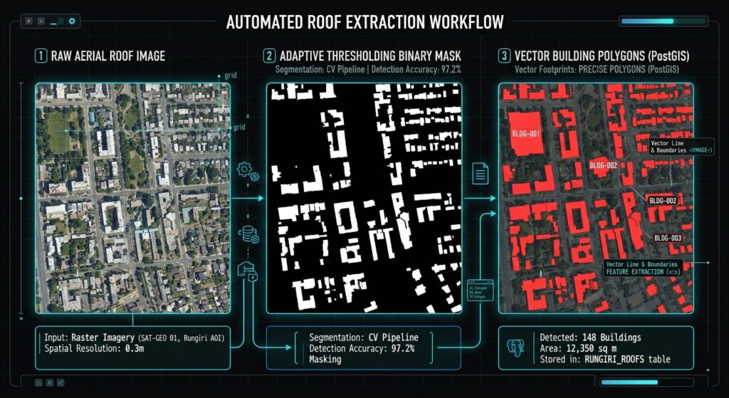
Visual inspection helps identify which stage is causing errors before you start changing parameters.

Add the following block after segmentation and contour filtering. It saves intermediate images and an overlay of accepted candidate contours.

# Save intermediate processing results.cv2.imwrite("debug_threshold.png", threshold_clean)cv2.imwrite("debug_edges.png", edges)cv2.imwrite("debug_candidates.png", combined_mask)# Draw retained contours on the enhanced RGB image.overlay = rgb.copy()cv2.drawContours(    overlay,    accepted_contours,    contourIdx=-1,    color=(255, 0, 0),    thickness=2)# OpenCV's image writer expects BGR channel order.overlay_bgr = cv2.cvtColor(    overlay,    cv2.COLOR_RGB2BGR)cv2.imwrite("footprints_preview.png", overlay_bgr)print("Diagnostic images saved.")

Expected outputs:

These are descriptions of the expected outputs, not actual results from a particular orthophoto. Their appearance depends on the imagery and parameter settings.

9. Limitations and fine-tuning

Problem 1: Tree shadows generate building candidates

Dark shadows can be classified in the same way as dark roofs, particularly when using inverse adaptive thresholding. Tree crowns can also have clear boundaries that resemble roof outlines.

What to try: Increase the adaptive block size if local thresholds respond too strongly to tiny variations. Adjust ADAPTIVE_C, compare bright and dark polarity, and reduce excessive edge dilation or morphological closing. Where multispectral imagery is available, vegetation indices can provide additional evidence for distinguishing vegetation from rooftops.

These changes may reduce false detections, but no single setting reliably separates every shadow from every roof.

Problem 2: Roof colors vary across the scene

A neighborhood may contain metal roofs, concrete slabs, red tiles, and dark roofing materials. A single threshold polarity can miss an entire roof class.

What to try: Test the bright and dark threshold settings separately. Examine debug_threshold.png and debug_candidates.png before selecting a setting. A more advanced classical approach could combine multiple candidate masks and color-based rules, although overlapping detections would then need to be resolved.

Problem 3: Adjacent buildings merge into one polygon

Closing operations connect short gaps in segmented regions. That is helpful for incomplete boundaries but can merge neighboring buildings when they are close together.

What to try: Reduce the kernel size or number of closing iterations. Inspect whether the merge occurs in the threshold mask or only after combining it with the edge map. Watershed segmentation or distance-transform-based splitting may help in some cases.

Problem 4: Footprints are jagged or excessively detailed

Image noise and roof textures can produce irregular contours even when the general roof extent is correct.

What to try: Increase SIMPLIFY_EPSILON_PX slightly to remove redundant points, or increase the Gaussian blur kernel if the input is noisy. Avoid aggressive simplification because it can distort small buildings and remove important corners.

Problem 5: The process is too slow for a large orthophoto

Large aerial images consume substantial memory when loaded as complete arrays. Several masks and intermediate images can multiply memory use.

What to try: Process the raster in windows or manageable tiles, using each window’s own geospatial transform to convert pixel contours to map coordinates. Add sufficient overlap between tiles so that buildings crossing tile boundaries are not truncated, and reconcile duplicate or fragmented features in the overlapping zones. The example in this article processes the complete raster at once.

Problem 6: The GeoPackage contains polygons but they are in the wrong location

The most common causes include incorrect source CRS metadata, using the wrong RGB band order, or applying an incorrect transform when converting contour coordinates.

What to try: Check src.crs, src.transform, and src.bounds. Confirm the vector layer’s CRS in QGIS and compare it with the raster. Never treat raw OpenCV pixel coordinates as longitude and latitude.

10. When should you move beyond OpenCV?

OpenCV is useful when you want a lightweight, interpretable workflow without preparing a labeled training dataset. However, it primarily detects local image characteristics rather than understanding the object being depicted.

For production-scale building extraction, consider a semantic segmentation model such as U-Net or a building-footprint segmentation model trained on aerial imagery. Such models can learn patterns associated with roofs, vegetation, and roads, including cases where simple color thresholds fail.

A hybrid workflow is also possible: use a segmentation model to identify building regions, then use OpenCV and Shapely to refine boundaries, eliminate small artifacts, simplify geometry, and prepare the results for GIS storage.

11. Summary

This tutorial demonstrated how to extract building footprints from aerial imagery using OpenCV and Python GIS libraries. The workflow reads a georeferenced GeoTIFF, performs contrast stretching and color-space conversion, applies adaptive thresholding and Canny edge detection, cleans candidate masks with morphology, converts contours to Shapely polygons, and exports the results to GeoPackage.

The essential distinction is between detecting image patterns and identifying buildings. The resulting layer can accelerate initial mapping, but its accuracy must be assessed against the original imagery and, where possible, reference footprints.

For practical GIS projects, begin with a small representative section of the orthophoto, tune the parameters, inspect the diagnostic images, and validate the output before processing an entire city or using the layer for cadastral or planning decisions.

Technical references

• OpenCV — Finding contours in your image

• Rasterio — Python Quickstart and georeferencing

• Rasterio — Coordinate transformations

• Shapely — Geometry operations and validation

• GeoPandas — Writing vector data to files