
Spatial Point Pattern Simulation and Monte Carlo Testing in Python
1. Introduction

Spatial Point Pattern Simulation Python methods provide a robust framework for evaluating whether an observed distribution differs significantly from a specified random spatial model. A map of disease cases, retail stores, crime incidents, wildlife sightings, or traffic accidents may reveal apparent spatial clusters. However, seeing points concentrated in one location does not necessarily mean that a meaningful spatial process produced the pattern. Some clustering can occur naturally through random variation, particularly when many points are observed within a limited study area.
Spatial point pattern simulation and Monte Carlo testing in Python provide a framework for evaluating whether an observed distribution differs significantly from a specified random spatial model.
Instead of relying only on visual interpretation, we generate many artificial point patterns under a null hypothesis, calculate spatial statistics for each simulated pattern, and compare those results against the observed data. This approach estimates how unusual the observed pattern would be if the null model were true.
For example, a public health researcher might ask whether recorded disease cases are more spatially concentrated than expected under complete spatial randomness (CSR). A retail analyst might investigate whether shop locations exhibit clustering beyond what would be expected if the same number of shops were distributed randomly across an eligible urban area.
This tutorial develops a reproducible workflow using Python, GeoPandas, SciPy, NumPy, and Matplotlib. It covers point simulation inside polygon boundaries, nearest-neighbor statistics, Ripley’s K, simulation envelopes, Monte Carlo p-values, and the interpretation of statistical significance.
2. Defining Complete Spatial Randomness (CSR)
Complete spatial randomness is a reference model for a spatial point pattern. Under a homogeneous Poisson point process, events occur independently, with a constant intensity across the study area.
The model has two related components:
-
Count variation: The number of events in an area \(A\) follows a Poisson distribution with expected count \(\lambda A\), where \(\lambda\) is the event intensity per unit area.
-
Spatial placement: Conditional on observing \(N\) events, their locations are independently and uniformly distributed over the study region.
This second formulation is particularly useful for testing clustering because it holds the observed number of points constant and randomizes their locations within the same study-area boundary.
The hypotheses
A typical CSR test evaluates:
The alternative hypothesis can be directional or two-sided. For example, a clustering test asks whether points are closer together than expected, while a regularity test asks whether points are more evenly spaced than expected.
CSR is a useful baseline, not a universal model of realistic human or environmental activity. If shops can only occur beside roads, or disease risk varies substantially across a region, uniform random placement may be an inappropriate null model. Rejecting CSR in these circumstances does not, by itself, establish the mechanism causing the pattern.
Why simulate instead of using only a theoretical distribution?
Real study areas have irregular boundaries, and spatial statistics can behave differently near those boundaries. Monte Carlo simulation lets us generate random point patterns within the actual study area and compare the observed statistic with the distribution produced under the chosen null hypothesis.
We will use two complementary statistics:
-
Mean nearest-neighbor distance: A single-number summary of how close each point is to its nearest neighboring point.
-
Ripley’s K function: A distance-dependent statistic that examines the accumulation of neighboring points over a range of spatial scales.
SciPy’s cKDTree supports efficient nearest-neighbor searches, making it suitable for
3. Environment setup
Install the required libraries
Use Python 3.10 or later and install the dependencies:
python -m pip install numpy scipy pandas geopandas shapely matplotlibThe libraries have the following roles:
| Library | Purpose |
|---|---|
| NumPy | Random number generation, array operations, and Monte Carlo calculations |
| SciPy | Efficient nearest-neighbor search and pairwise distance calculations |
| GeoPandas | Reading spatial datasets and managing point and polygon layers |
| Shapely | Polygon containment tests and spatial geometry operations |
| Matplotlib | Plotting observed patterns and simulation envelopes |
| pandas | Organizing statistical outputs into tables and CSV files |
Prepare the input data
For a real study, prepare two spatial datasets:
study_area.gpkg — a polygon or multipolygon defining the area in which events could be observed.
observed_points.gpkg — a point layer containing the locations of the observed events.
Both layers need defined coordinate reference systems. The study area should use a suitable projected CRS so that distances and area are measured in meaningful linear units rather than degrees of longitude and latitude.
The tutorial’s main script defaults to a synthetic example so it can run without external data. You can switch to your own datasets by changing one configuration setting.
4. Step-by-step Python workflow
Step 1 — Define the study area and observed point pattern
Start by importing the libraries and configuring the Monte Carlo experiment.
We will use 999 simulations. With the standard plus-one Monte Carlo p-value formula, this gives a minimum attainable one-sided p-value of \(1/1000 = 0.001\). A smaller number of simulations, such as 99, is useful for exploratory analysis, but provides less precise tail probabilities.
The synthetic example contains 160 deliberately clustered points in an irregular polygon. This gives us a reproducible way to demonstrate whether the methods detect a departure from CSR.
import numpy as npimport pandas as pdimport geopandas as gpdimport matplotlib.pyplot as pltfrom shapely.geometry import Point, Polygonfrom shapely.ops import unary_unionfrom scipy.spatial import cKDTreefrom scipy.spatial.distance import pdist# ---------------------------------------------------------# Configuration# ---------------------------------------------------------SEED = 20261020N_SIMULATIONS = 999# Example distance range in metres for the synthetic dataset.# Change these distances to suit your research question.R_MIN = 100.0R_MAX = 1800.0N_RADII = 30# Distance at which to report a pointwise Ripley's K p-value.REPORT_RADIUS = 500.0# True: use synthetic teaching data.# False: read your own GeoPackage layers.USE_DEMO_DATA = Truerng = np.random.default_rng(SEED)# ---------------------------------------------------------What this step establishes: The analysis window defines where random points may occur. Each simulation will preserve the observed number of events while generating fresh, independent locations inside that same boundary.
The synthetic polygon uses EPSG:32737 solely as a projected metric coordinate system for the demonstration. For real data, retain the appropriate local projected CRS for your study region.
The rejection-sampling function also handles irregular polygon boundaries: points falling outside the actual polygon are discarded, including points that fall into indentations or holes.
Step 2 — Plot and inspect the observed pattern
Before calculating any statistics, plot the events and study-area boundary.
fig, ax = plt.subplots(figsize=(8, 7))study_area_gdf.boundary.plot( ax=ax, color="black", linewidth=1.5)observed_gdf.plot( ax=ax, markersize=12, alpha=0.8)ax.set_title( f"Observed Spatial Point Pattern (N={len(observed_xy)})")ax.set_xlabel(f"Easting ({distance_unit})")ax.set_ylabel(f"Northing ({distance_unit})")ax.set_aspect("equal", adjustable="box")plt.tight_layout()plt.savefig( "observed_point_pattern.png", dpi=180, bbox_inches="tight")plt.show()The resulting map should display the observed event locations within the study boundary. In the synthetic dataset, four concentrations of points should be visible.
Visual inspection is useful for finding obvious data-quality problems, such as events falling outside the intended study area. However, the apparent strength of clustering is not a substitute for statistical testing.
Step 3 — Calculate the mean nearest-neighbor distance
The mean nearest-neighbor distance provides a simple statistic for evaluating local concentration.
For each observed point \(i\), calculate the distance to its closest other point:
Then calculate the mean:
Smaller values generally indicate closer spacing between neighboring points, while larger values indicate wider spacing.
SciPy’s cKDTree.query() can efficiently retrieve the two closest results for each point. The first is the point itself, with distance zero; the second is its nearest neighbor.
def mean_nearest_neighbor_distance(xy): """ Return the mean nearest-neighbor distance. Parameters ---------- xy : array-like, shape (n_points, 2) Coordinates in a projected CRS. Returns ------- float Mean distance to the nearest other point. """ if len(xy) < 2: raise ValueError("At least two points are required.") tree = cKDTree(xy) # k=2 includes each point and its nearest other point. distances, indices = tree.query(xy, k=2) nearest_distances = distances[:, 1] return float(nearest_distances.mean())# Calculate the statistic for the observed point pattern.observed_nn = mean_nearest_neighbor_distance(observed_xy)print( f"Observed mean nearest-neighbor distance: " f"{observed_nn:.2f} {distance_unit}")The result is one distance value for the entire observed point pattern.
At this stage, that value alone does not establish statistical significance. Whether a mean distance is unusually small depends on the study-area geometry, point count, and the variability expected under CSR.
Step 4 — Calculate Ripley’s K function
Nearest-neighbor distance is useful for summarizing local spacing, but it cannot fully describe how a pattern changes with distance. Ripley’s K function evaluates the accumulation of neighboring point pairs over a range of distances.
For a homogeneous Poisson process in an unbounded plane, the theoretical K function is:
where \(r\) is the search distance.
Intuitively, K measures how many other points accumulate within a distance \(r\), after accounting for the overall point density. Values larger than expected under CSR are consistent with clustering at that scale; smaller values are consistent with regularity or inhibition.
For this implementation, we calculate an uncorrected estimator of K:
Here, \(|W|\) is the study-area size, and the indicator equals one whenever a pair of distinct points is within the specified distance.
The estimator below uses SciPy’s pdist() to calculate all unique pairwise distances and numpy.searchsorted() to count the pairs within each radius.
def ripley_k_uncorrected(xy, radii, area): """ Calculate an uncorrected Ripley's K estimate at each radius. All coordinates and radii must use the same projected units. Boundary effects are assessed using the Monte Carlo null model. """ n = len(xy) if n < 2: raise ValueError("At least two points are required.") # Each unordered pair appears once in pdist(). pair_distances = np.sort( pdist(xy, metric="euclidean") ) # Count unordered pairs at or below each radius. pair_counts = np.searchsorted( pair_distances, radii, side="right" ) # Ripley's estimator uses ordered pairs, hence 2 * pair_counts. k_values = ( area * 2.0 * pair_counts / (n * (n - 1)) ) return k_values# Define the observed distance-dependent statistic.observed_k = ripley_k_uncorrected( observed_xy,This estimator is intentionally uncorrected for boundaries. That choice makes the example easier to implement and understand, but its observed K values should not be compared naively with \(\pi r^2\) near irregular boundaries.
Instead, we use the same estimator for the observed data and every simulated dataset inside the identical study window. The simulation distribution therefore reflects the estimator’s boundary effects under the specified null model.
For research requiring direct interpretation of conventional K curves or comparison with theoretical CSR curves, consider an edge-corrected estimator and use the same edge correction in every simulation.
Step 5 — Generate Monte Carlo point patterns
We can now simulate 999 datasets under conditional CSR.
For each repetition:
-
Generate the same number of points as in the observed pattern.
-
Place them independently and uniformly within the study-area polygon.
-
Calculate the mean nearest-neighbor distance.
-
Calculate Ripley’s K at each selected radius.
-
Store both sets of statistics for comparison.
This is a conditional CSR test because the number of events \(N\) remains fixed. It tests their spatial arrangement rather than whether the overall number of events is unusually large or small.
# Number of observed events is held fixed under conditional CSR.n_points = len(observed_xy)# Arrays to store results from every simulation.simulated_nn = np.empty(N_SIMULATIONS, dtype=float)simulated_k = np.empty( (N_SIMULATIONS, len(radii)), dtype=float)for i in range(N_SIMULATIONS): # Generate a new uniformly random pattern in the same window. simulated_xy = sample_uniform_in_polygon( window, n_points, rng ) # Statistic 1: mean nearest-neighbor distance. simulated_nn[i] = mean_nearest_neighbor_distance( simulated_xy ) # Statistic 2: Ripley's K at every radius. simulated_k[i, :] = ripley_k_uncorrected( simulated_xy, radii, study_area )print("Completed simulations:", N_SIMULATIONS)print(Each row of simulated_k contains a complete Ripley’s K curve from one simulated pattern. The array therefore represents the null distribution of the statistic across both distance scales and simulated realizations.
A key advantage of this approach is that simulations preserve the same study boundary and the same event count. Random patterns are not generated over the entire rectangular bounding box without constraint.
For efficient point-pattern simulation inside arbitrary spatial regions, the pointpats package also offers Poisson and other spatial point-process simulation methods.
Step 6 — Calculate Monte Carlo p-values
A Monte Carlo test compares the observed statistic against the values obtained from simulated patterns.
For a clustering alternative based on nearest-neighbor distance, unusually small observed distances provide evidence against CSR. A one-sided Monte Carlo p-value is:
where \(M\) is the number of simulations.
The plus-one adjustment prevents an estimated p-value of exactly zero and accounts for the observed pattern as one of the competing realizations in the Monte Carlo ranking.
For Ripley’s K, we calculate pointwise upper-tail probabilities at each distance to assess clustering, and lower-tail probabilities to assess regularity.
# ---------------------------------------------------------# Nearest-neighbor Monte Carlo test# ---------------------------------------------------------# Clustering: observed NN distance is unusually small.p_nn_cluster = ( 1 + np.count_nonzero(simulated_nn <= observed_nn)) / (N_SIMULATIONS + 1)# Regularity: observed NN distance is unusually large.p_nn_regular = ( 1 + np.count_nonzero(simulated_nn >= observed_nn)) / (N_SIMULATIONS + 1)# A simple two-sided summary based on the smaller tail.p_nn_two_sided = min( 1.0, 2.0 * min(p_nn_cluster, p_nn_regular))mean_simulated_nn = float(simulated_nn.mean())# Descriptive ratio: observed spacing / simulated CSR spacing.nn_ratio = observed_nn / mean_simulated_nn# ---------------------------------------------------------# Ripley's K pointwise Monte Carlo tests# ---------------------------------------------------------# Upper-tail probability: evidence for clustering.p_k_cluster = ( 1 + np.sum( simulated_k >= observed_k[None, :], axis=0 )Interpreting the nearest-neighbor results
The nearest-neighbor ratio compares the observed mean spacing with the average spacing from CSR simulations.
-
A ratio below 1 indicates that the observed points are closer together on average than the CSR simulations.
-
A ratio above 1 indicates wider spacing than the CSR simulations.
-
A small clustering p-value indicates that a mean distance at least this small is unusual under the specified CSR null model.
A small p-value does not tell you why clustering occurred. It only indicates incompatibility with the chosen reference model at the specified significance level.
Interpreting Ripley’s K p-values
Ripley’s K gives a different view because its statistic changes with \(r\). A small upper-tail p-value at a particular distance indicates that the observed K is unusually large compared with CSR simulations at that distance. A small lower-tail p-value indicates an unusually small K.
Because the K test examines many distances, interpreting the entire curve requires care. Pointwise p-values assess one distance at a time. They do not automatically control the chance of finding at least one significant result across all inspected distances.
Step 7 — Build the Monte Carlo simulation envelope
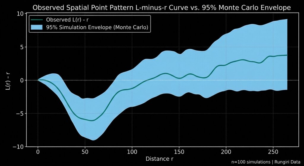
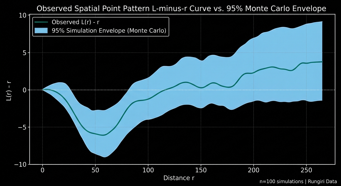
A simulation envelope provides a visual comparison between the observed spatial statistic and the range of values generated under CSR.
For every simulation, transform K to the commonly used L-function form:
The transformed quantity \(L(r)-r\) is easier to interpret in distance units. Positive departures are often associated with clustering, while negative departures are often associated with regularity.
# Transform K into L(r) - r for easier visual interpretation.observed_l = ( np.sqrt(np.maximum(observed_k, 0) / np.pi) - radii)simulated_l = ( np.sqrt(np.maximum(simulated_k, 0) / np.pi) - radii[None, :])# Pointwise 95% simulation envelope.lower_envelope, upper_envelope = np.quantile( simulated_l, [0.025, 0.975], axis=0)# Plot the observed curve against the envelope.fig, ax = plt.subplots(figsize=(9, 5.5))ax.fill_between( radii, lower_envelope, upper_envelope, alpha=0.25, label="95% pointwise CSR envelope")ax.plot( radii, observed_l, linewidth=2, label="Observed L(r) - r")Expected figure: an observed curve surrounded by a shaded pointwise simulation envelope. The actual curves and envelope widths depend on the data and simulation settings.
The figure should be interpreted as follows:
-
Observed curve above the upper envelope: Evidence of clustering at the corresponding distance, according to the pointwise CSR test.
-
Observed curve below the lower envelope: Evidence of greater spacing or inhibition at that distance.
-
Observed curve inside the envelope: No pointwise departure detected at that distance at the nominal envelope level.
The zero reference is a useful visual guide, but this implementation uses an uncorrected K estimator. For an irregular finite study window, the simulation envelope—not the zero line—is the primary reference for inference.
Pointwise envelopes should not be confused with simultaneous envelopes. When a researcher searches across many distance scales, a nominal 95% pointwise envelope does not guarantee a 5% overall error rate. This distinction is important in spatial point-pattern inference.
Step 8 — Calculate an overall Monte Carlo test across distance scales
An overall test is useful when the research question asks whether the observed point pattern departs from CSR anywhere within a predefined range of distances.
A simple approach is to calculate a maximum standardized deviation of each K curve from the ensemble mean. A curve with large positive or negative departures at any selected distance receives a high score.
To preserve symmetry under the null hypothesis, the code calculates the center and standard deviation using the complete ensemble, including the observed curve and the simulated curves. The observed score is then ranked against the simulated scores to obtain a global Monte Carlo p-value.
# ---------------------------------------------------------# Global Monte Carlo test using maximum standardized deviation# ---------------------------------------------------------# Include the observed K curve and every simulated K curve.all_k = np.vstack([ observed_k[None, :], simulated_k])# Calculate a common reference centre and scale at each radius.center_k = all_k.mean(axis=0)scale_k = all_k.std(axis=0, ddof=1)# Protect against zero-variance distances.scale_k = np.where(scale_k > 0, scale_k, 1.0)# Standardize each curve against the common reference.standardized_curves = ( all_k - center_k[None, :]) / scale_k[None, :]# Each pattern gets one statistic:# the largest absolute standardized departure over all radii.global_scores = np.max( np.abs(standardized_curves), axis=1)observed_global_score = global_scores[0]simulated_global_scores = global_scores[1:]# Global two-sided Monte Carlo p-value.p_global_k = ( 1 + np.count_nonzero( simulated_global_scores >= observed_global_scoreThis maximum-deviation test asks whether the observed curve departs unusually far from the ensemble reference at one or more of the selected distances. Because the statistic is calculated symmetrically across the ensemble, its Monte Carlo ranking can be used as an overall test under the conditional CSR null.
The global test is the more appropriate result when the scientific claim concerns departure across the entire predefined range of distances. The pointwise envelopes remain useful for visualizing where departures occur, but they should not be treated as proof that every inspected distance has been independently tested at a 5% family-wise error rate.
For formal publication-level work, researchers may also use established global rank-envelope procedures designed specifically for functional spatial statistics.
Step 9 — Export the statistical results
Store the Ripley’s K values, transformed curves, simulation envelopes, and pointwise p-values in a CSV table. This makes it easier to inspect results, generate publication figures, and document the experiment.
# Create a table with one row per distance scale.results = pd.DataFrame({ "distance": radii, "K_observed": observed_k, "L_minus_r_observed": observed_l, "L_minus_r_lower_95_pointwise": lower_envelope, "L_minus_r_upper_95_pointwise": upper_envelope, "p_cluster_upper_pointwise": p_k_cluster, "p_regular_lower_pointwise": p_k_regular, "p_two_sided_pointwise": p_k_two_sided,})results.to_csv( "ripley_mc_results.csv", index=False)print("Saved Ripley's K results to ripley_mc_results.csv")The CSV contains the observed statistic and its pointwise Monte Carlo comparison at each distance. Report the global K-function p-value separately because it summarizes the departure across the selected distance range rather than at one particular radius.
5. Limitations and practical considerations
Choosing the right null model
The assumption of homogeneous CSR is often the most important limitation. Retail stores, disease cases, and road incidents may naturally follow population density, transportation networks, or environmental suitability. If the process intensity varies across space, a homogeneous CSR test may detect that variation rather than a distinct clustering mechanism.
Consider testing against an inhomogeneous Poisson process or another domain-appropriate null model when there is a justified reason to expect spatially varying intensity. Where the research question concerns clustering beyond a known pattern of exposure or accessibility, that structure should be reflected in the null model.
Study-area boundaries and edge effects
Points near the boundary have less surrounding area available for neighboring observations. This can bias spatial statistics that count nearby points.
The example addresses the issue by simulating points inside the exact study window and using the same K estimator for both observed and simulated patterns. An edge-corrected K estimator may be preferable for analyses intended to compare with the theoretical Poisson benchmark.
Simulation count and statistical resolution
With 99 simulations, the smallest one-sided p-value attainable using the plus-one formula is 0.01. With 999 simulations, it is 0.001. More simulations improve Monte Carlo resolution but require additional computation.
Choose the number of simulations based on the significance level and precision required for the study. Use a fixed random seed during development to make your results reproducible, and document the final seed and number of simulations in your methods.
Interpreting a significant result
A statistically significant result indicates that the observed pattern is unusual under the chosen null model. It does not, on its own, prove that a particular causal mechanism produced the pattern.
For example, statistically significant clustering of disease cases does not establish a localized source of infection without further investigation of population distribution, exposure, surveillance practices, and other relevant factors.
6. Conclusion and practical takeaways for research papers
Monte Carlo methods provide an accessible and flexible way to assess spatial clustering beyond visual inspection. By generating randomized patterns within a fixed study area, researchers can estimate the distribution of spatial statistics under a defensible null hypothesis and evaluate whether observed patterns depart from it.
The workflow in this tutorial implements two complementary approaches: a nearest-neighbor test for overall local spacing and Ripley’s K for examining departures over a range of distances. Pointwise envelopes identify potential scales of clustering or regularity, while the global maximum-deviation test provides an overall test across the selected distance range.
For a research paper, document the study-area boundary, CRS and distance units, the conditional or unconditional CSR assumption, the statistic and distance range, the number of simulations, the Monte Carlo p-value method, and whether the reported inference is pointwise or global. Include the seed and software versions to support reproducibility.
Most importantly, interpret statistical significance relative to the null model rather than as proof of a causal explanation. A well-designed spatial test begins not with the number of points or the number of simulations, but with a clear statement of what random spatial process the observed pattern is being compared against.