
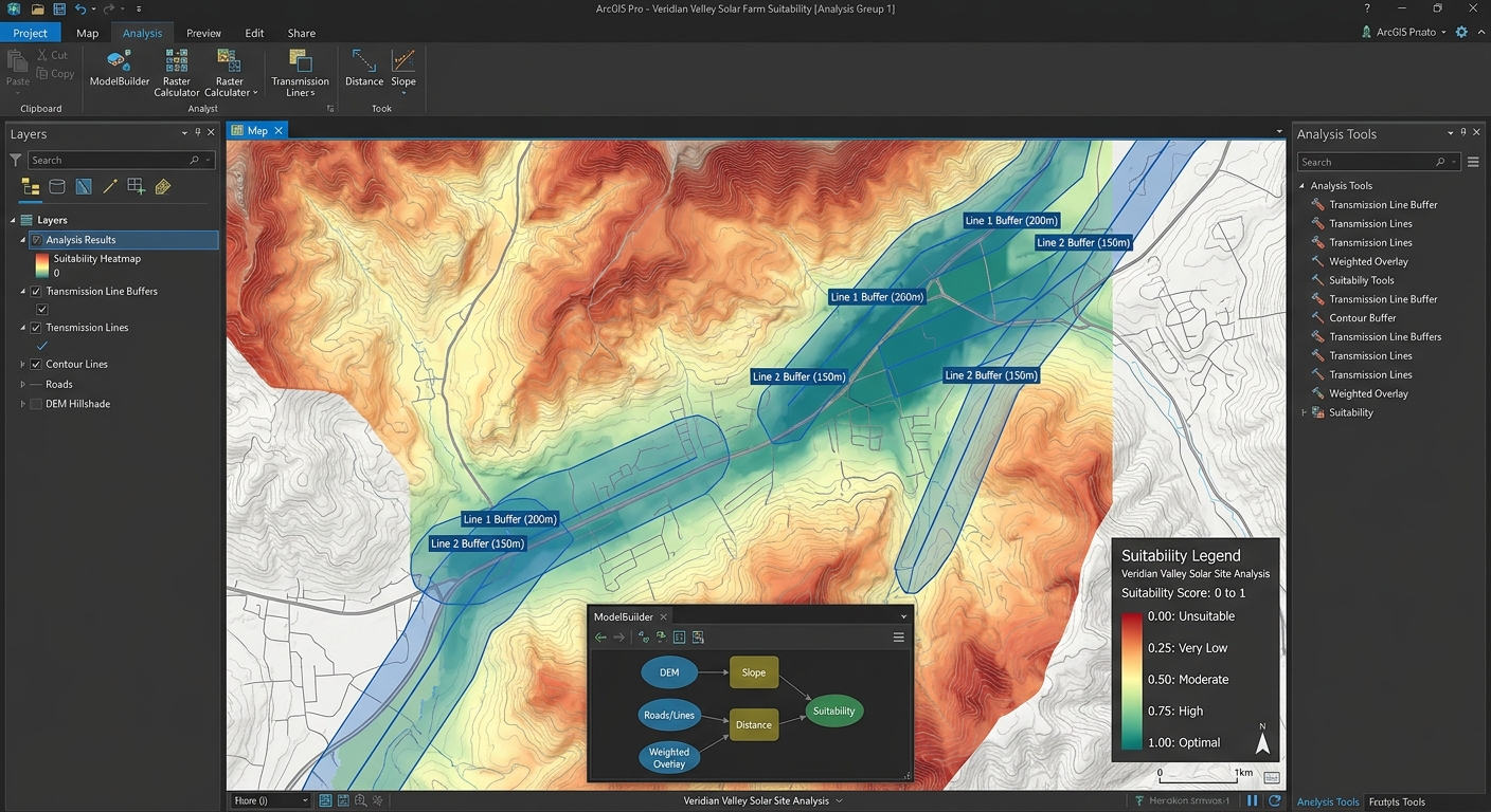
Fuzzy Logic in GIS Site Suitability: Moving Beyond Binary Constraints
Introduction
Traditional GIS site suitability analysis often relies on Boolean logic, where every location is classified as either suitable (1) or unsuitable (0). This approach is straightforward and easy to implement, but it can oversimplify geographic reality.
Consider a hospital site-selection rule requiring a location to be at least 500 m from a major road. Under Boolean logic:
- 499 m → unsuitable (
0) - 500 m → suitable (
1) - 501 m → suitable (
1)
The problem is obvious: a one-metre difference can produce a complete change in suitability.
Real-world suitability rarely behaves this way. A site 499 m from a road is not necessarily fundamentally different from one 500 m away. Instead, suitability usually changes gradually.
This is where Fuzzy Logic GIS Site Suitability Analysis becomes valuable. Rather than forcing geographic variables into binary categories, fuzzy logic converts them into continuous membership values between 0 and 1.
0= completely unsuitable0.25= very low suitability0.50= moderate suitability0.75= high suitability1.00= fully suitable/optimal
The result is a continuous suitability model that better represents uncertainty, gradual transitions, and expert knowledge.
1. Boolean vs. Fuzzy Site Suitability
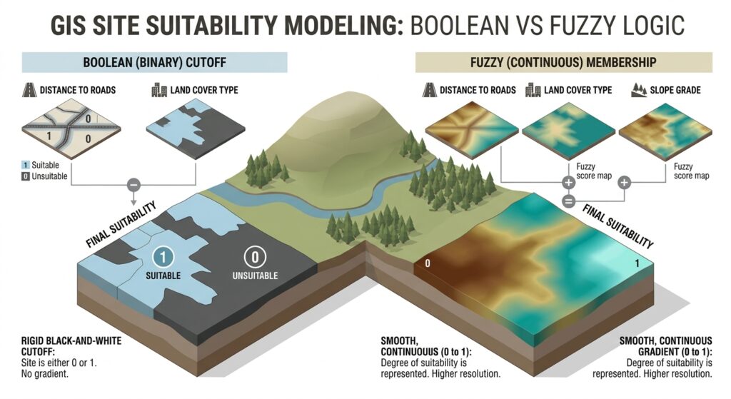
Before implementing fuzzy logic, it is important to understand exactly what changes.
Boolean approach
Suppose you are selecting a solar-farm location using three constraints:
- Slope ≤ 10°
- Distance from roads ≥ 500 m
- Elevation between 1,000 and 2,000 m
A Boolean model might be written as:
\[ S = C_1 \times C_2 \times C_3 \]
where every constraint has a value of either 0 or 1.
A location satisfying all three receives:
\[ 1 \times 1 \times 1 = 1 \]
A location failing one receives:
\[ 1 \times 0 \times 1 = 0 \]
That means one failed criterion can completely eliminate a location.
Fuzzy approach
Fuzzy logic instead represents each criterion using a membership function:
\[ \mu_i(x) \in [0,1] \]
where:
- \(\mu_i(x)=0\) means no membership
- \(\mu_i(x)=1\) means complete membership
- intermediate values represent partial membership.
A location with memberships of:
- slope = 0.85
- road distance = 0.70
- elevation = 0.95
is not simply classified as “suitable.” Its suitability characteristics are retained numerically.
This distinction is fundamental to Boolean vs fuzzy logic spatial analysis.
2. How Fuzzy Logic Works in GIS
The core process consists of three stages:
Raw geographic variable → Fuzzy membership transformation → Fuzzy overlay
For example:
Slope Raster
     ↓
Fuzzy Membership Function
     ↓
Slope Membership Raster
     ↓
0 ─────────────── 1
Unsuitable       Optimal
Instead of directly combining the raw slope values with distance and elevation, each variable is first transformed into a common suitability scale.
This makes fundamentally different variables comparable.
For example:
| Criterion | Original measurement | Fuzzy membership |
|---|---|---|
| Slope | 0–45° | 0–1 |
| Road distance | 0–5,000 m | 0–1 |
| Elevation | 500–3,000 m | 0–1 |
| Solar radiation | 0–8 kWh/m² | 0–1 |
Once standardized, these layers can be combined using fuzzy overlay operators.
3. Fuzzy Membership Functions GIS
The membership function is one of the most important decisions in a fuzzy suitability model.
It defines how rapidly suitability changes as an attribute changes.
Common fuzzy membership functions in GIS include:
- Linear
- Small
- Large
- Gaussian
- Sigmoidal
3.1 Linear Membership
A linear function is appropriate when suitability changes gradually and predictably.
For a variable where larger values are better:
\[ \mu(x)= \begin{cases} 0 & x\leq a\\ \frac{x-a}{b-a} & a<x<b\\ 1 & x\geq b \end{cases} \]
where:
- \(a\) = minimum acceptable value
- \(b\) = value at which full suitability is reached.
For example, suppose solar radiation below 4 kWh/m²/day is unsuitable and 6 kWh/m²/day or greater is optimal.
| Solar radiation | Membership |
|---|---|
| 3.5 | 0.00 |
| 4.0 | 0.00 |
| 4.5 | 0.25 |
| 5.0 | 0.50 |
| 5.5 | 0.75 |
| 6.0 | 1.00 |
This is useful when the transition from unsuitable to optimal is approximately linear.
3.2 Small Membership Function
A Small function assigns greater suitability to smaller values.
This is useful for criteria such as:
- Distance to electricity infrastructure
- Distance to roads
- Slope
- Travel time
- Development cost
For example, if a solar farm should be relatively close to transmission infrastructure, smaller distance values receive higher membership.
Conceptually:
Membership
1.0 |████████
    |███████
    |█████
    |███
0.0 |________________
       Increasing distance
The exact shape can be adjusted depending on the decision-maker’s assumptions.
3.3 Large Membership Function
The Large function reverses the relationship.
It is appropriate when increasing values represent increasing suitability.
Examples include:
- Solar radiation
- Renewable-energy potential
- Ground stability
- Agricultural productivity
- Distance from environmentally sensitive areas
For example:
\[ x \uparrow \quad \Rightarrow \quad \mu(x) \uparrow \]
A location farther away from a protected ecosystem might therefore receive progressively higher suitability.
3.4 Gaussian Membership
A Gaussian function is useful when there is an optimal central value and suitability decreases in both directions.
A common formulation is:
$$y = e^{-\frac{(x-50)^2}{2(15)^2}} \{0 \le x \le 100\}$$
where:
- \(c\) = optimal value
- \(\sigma\) = spread of the suitability curve.
For example, suppose a particular elevation range is preferred for a development project.
Extremely low elevations may be unsuitable, while extremely high elevations may also be unsuitable. The best locations occur around the preferred elevation.
20406080100607080901000.20.40.60.8−0.2−0.4−0.6
This makes Gaussian membership particularly useful for variables where “closer to an optimum” is more realistic than simply “higher is better” or “lower is better.”
3.5 Sigmoidal Membership
A sigmoidal function creates a smooth S-shaped transition between unsuitable and suitable conditions.
A conceptual formulation is:
\[ \mu(x)=\frac{1}{1+e^{-k(x-c)}} \]
where:
- \(c\) controls the midpoint
- \(k\) controls the steepness.
Sigmoidal functions are useful when suitability changes slowly at first, then rapidly around a critical region, before approaching maximum suitability.
This can be more realistic than an abrupt Boolean threshold.
4. Step-by-Step Fuzzy Site Suitability Workflow
The following workflow can be implemented using raster analysis tools in QGIS or ArcGIS Pro.
The exact interface names differ between the two platforms, but the conceptual workflow is essentially the same.
Step 1: Define the Decision Problem
Start by identifying the actual decision rather than immediately choosing GIS tools.
For example:
Identify locations suitable for constructing a new solar farm.
Potential criteria could include:
- Slope
- Solar radiation
- Distance to transmission lines
- Distance to roads
- Land-use restrictions
- Elevation
- Protected areas
Separate the criteria into two categories:
Continuous suitability criteria
These benefit from fuzzy membership:
- Slope
- Distance
- Solar radiation
- Elevation
- Travel time
Hard constraints
Some areas genuinely should remain excluded.
Examples:
- Protected areas
- Existing buildings
- Water bodies
- Airport safety zones
- Legally restricted land
This is important: fuzzy logic does not mean eliminating every hard constraint.
A hybrid model can be more appropriate:
\[ S_{final}=H\times F \]
where:
- \(H\) = binary hard-constraint mask
- \(F\) = fuzzy suitability surface.
5. Step 2: Prepare the Spatial Data
Convert your input datasets into compatible raster layers.
For example:
Road network
     ↓
Distance raster

Elevation
     ↓
Slope raster

Solar radiation
     ↓
Solar resource raster

Protected areas
     ↓
Binary exclusion raster
Before performing raster calculations, ensure that the layers have compatible:
- Coordinate reference systems
- Cell sizes
- Spatial extents
- Alignment
- NoData handling
For a serious MCDA project, inconsistent raster alignment can introduce errors that have nothing to do with the fuzzy model itself.
6. Step 3: Define Fuzzy Membership Parameters
This is where the analytical judgment enters the model.
Suppose you are evaluating solar-farm sites.
Criterion A: Slope
Perhaps:
- ≤ 3° = optimal
- 3–15° = progressively less suitable
- ≥ 15° = unsuitable
You could therefore construct a Small or declining sigmoidal membership function.
Criterion B: Distance to transmission line
Perhaps:
- 0–500 m = highly suitable
- 500–2,000 m = increasingly less suitable
-
2,000 m = low suitability
A Small-type membership function would be appropriate.
Criterion C: Solar radiation
Perhaps:
- <4 kWh/m²/day = poor
- 4–6 = increasingly suitable
- ≥6 = optimal
A Large or linear membership function could be used.
The critical point is that these thresholds are now parameters of a continuous curve, rather than a single on/off switch.
7. Step 4: Create Fuzzy Membership Rasters
Each raw raster must be transformed independently.
For example:
Slope raster
      ↓
Fuzzy Small
      ↓
Slope_Fuzzy

Distance raster
      ↓
Fuzzy Small
      ↓
Distance_Fuzzy

Solar radiation
      ↓
Fuzzy Large
      ↓
Solar_Fuzzy
In QGIS, this can be implemented using raster calculator expressions or suitable GRASS/SAGA processing tools, depending on the workflow and installed providers.
In ArcGIS Pro, fuzzy membership tools are available through the Spatial Analyst workflow.
The important output is not the original measurement but the standardized membership surface:
\[ 0 \leq \mu(x) \leq 1 \]
8. Step 5: Apply Fuzzy Overlay Operators
Once the individual membership rasters have been created, combine them.
This is where fuzzy overlay differs significantly from simply adding standardized layers.
Fuzzy AND
Fuzzy AND generally emphasizes the least suitable criterion.
A common implementation is:
\[ \mu_{AND}=\min(\mu_1,\mu_2,\ldots,\mu_n) \]
Suppose:
\[ \mu_1=0.9,\quad \mu_2=0.7,\quad \mu_3=0.8 \]
Then:
\[ \mu_{AND}=0.7 \]
This is useful when all criteria must be reasonably strong.
Fuzzy OR
Fuzzy OR emphasizes the most favorable criterion:
\[ \mu_{OR}=\max(\mu_1,\mu_2,\ldots,\mu_n) \]
For:
\[ 0.9,\ 0.7,\ 0.8 \]
the result is:
\[ \mu_{OR}=0.9 \]
This represents a more permissive decision rule.
However, be careful: a high result under fuzzy OR does not necessarily mean that a location performs well across all criteria.
Fuzzy Product
Fuzzy Product combines membership values multiplicatively:
\[ \mu_{product}=\prod_{i=1}^{n}\mu_i \]
For three criteria:
\[ 0.9\times0.7\times0.8=0.504 \]
This operator is more restrictive than simply averaging the criteria.
A moderately weak criterion can substantially reduce the final score.
Fuzzy Sum
Fuzzy Sum uses a probabilistic-style combination:
\[ \mu_{sum}=1-\prod_{i=1}^{n}(1-\mu_i) \]
For:
\[ 0.9,\ 0.7,\ 0.8 \]
the result is:
\[ 1-(0.1)(0.3)(0.2)=0.994 \]
This can generate very high values when multiple criteria contribute positively.
Therefore, fuzzy sum should not automatically be interpreted as “more accurate.” It represents a different assumption about how evidence contributes to suitability.
9. Comparing Fuzzy and Boolean Results
This comparison is one of the most valuable parts of the workflow.
Imagine a traditional rule:
Slope must be ≤ 10°.
A Boolean classification might produce:
Slope ≤ 10°  → 1
Slope > 10°  → 0
The map contains an abrupt boundary.
The fuzzy model might instead produce:
0°–3°       → 1.00
3°–6°       → 0.85
6°–8°       → 0.65
8°–10°      → 0.40
10°–12°     → 0.20
>12°        → 0.00
Now the spatial transition is gradual.
Why this matters
Consider two neighboring cells:
| Slope | Boolean | Fuzzy |
|---|---|---|
| 9.9° | 1 | 0.42 |
| 10.0° | 1 | 0.40 |
| 10.1° | 0 | 0.38 |
The Boolean model treats 10.0° and 10.1° as fundamentally different.
The fuzzy model recognizes that they are practically similar.
10. Practical Case Study: Solar Farm Site Selection
Let’s construct a simplified solar-farm suitability model.
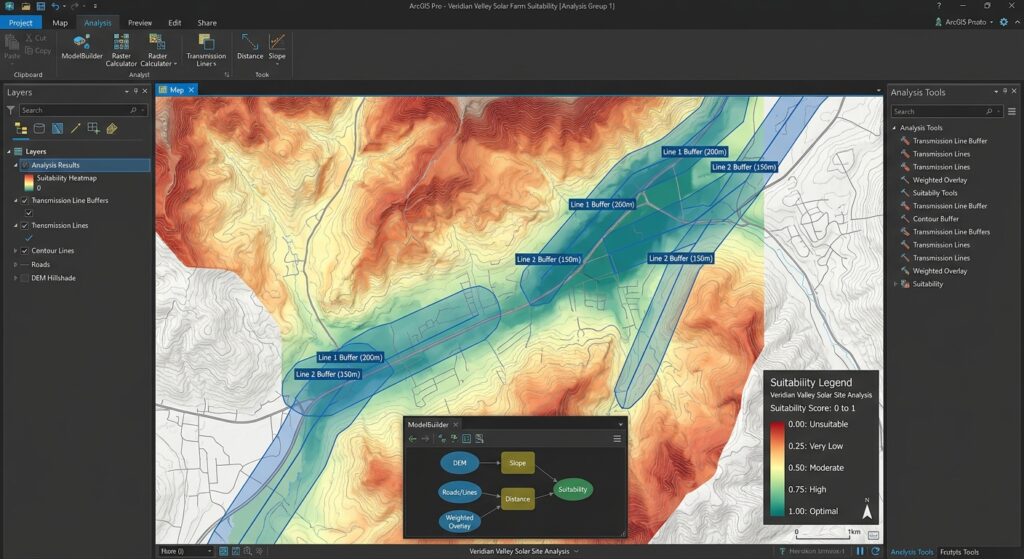
Objective
Identify areas with high potential for solar-farm development.
Criteria
| Criterion | Preference | Membership |
|---|---|---|
| Slope | Lower is better | Small |
| Solar radiation | Higher is better | Large |
| Distance to transmission | Lower is better | Small |
| Protected areas | Exclude | Boolean |
The workflow becomes:
                  ┌── Slope ────────→ Fuzzy Small ───┐
                  │                                    │
Input datasets ───┼── Solar radiation → Fuzzy Large ──┼→ Fuzzy Overlay
                  │                                    │
                  └── Transmission distance → Small ──┘

Protected areas ─────────────────────────────→ Hard Constraint
                                                    │
                                                    ↓
                                    Final Suitability Surface
Suppose a particular cell has:
- Slope membership = 0.85
- Solar membership = 0.90
- Transmission membership = 0.70
Using fuzzy product:
\[ S=0.85\times0.90\times0.70 \]\[ S=0.5355 \]
The location therefore has a suitability score of approximately 0.54 before applying the hard constraint.
If that cell falls inside a protected area:
\[ S_{final}=0 \]
If it does not:
\[ S_{final}=0.5355 \]
This produces a model that combines continuous preferences with absolute exclusions.
11. Implementing the Workflow in QGIS
A practical QGIS workflow could look like this:
A. Generate distance rasters
Use your road or transmission-line layer to create a distance raster.
B. Calculate terrain variables
From a DEM, derive:
- Slope
- Aspect
- Elevation
C. Standardize each variable
Use Raster Calculator or an appropriate processing algorithm to transform raw values into 0–1 membership values.
For example, a simple increasing linear transformation can be expressed as:
("solar@1" - 4) / (6 - 4)You would normally also constrain the output to the 0–1 range.
D. Combine membership layers
For a conservative fuzzy AND:
minimum(
    "slope_fuzzy@1",
    "solar_fuzzy@1",
    "distance_fuzzy@1"
)
For fuzzy product:
"slope_fuzzy@1"
*
"solar_fuzzy@1"
*
"distance_fuzzy@1"
The exact syntax can vary depending on layer names and the QGIS processing context, so validate the expression against the raster metadata before running it across a large project.
E. Apply hard constraints
Finally, multiply the fuzzy suitability surface by the binary exclusion mask.
"fuzzy_suitability@1"
*
"constraint_mask@1"
The result is a continuous suitability raster containing values from 0 to 1.
12. Implementing the Workflow in ArcGIS Pro
In ArcGIS Pro, the workflow can be organized around the Spatial Analyst tools.
A typical sequence is:
- Prepare input rasters.
- Generate distance and terrain variables.
- Apply Fuzzy Membership.
- Select an appropriate membership function.
- Specify the required parameters.
- Generate membership rasters.
- Apply Fuzzy Overlay.
- Compare the resulting surface with a Boolean model.
- Apply absolute exclusion constraints.
- Reclassify the final continuous surface into planning categories if necessary.
For example:
Fuzzy Membership
       ↓
Slope_Fuzzy
       ↓
                ┌──────────────┐
Solar_Fuzzy ───→│ Fuzzy Overlay│──→ Suitability
                └──────────────┘
Distance_Fuzzy ────────↑
One advantage of this approach is that the fuzzy membership and overlay stages remain conceptually separate. You can therefore change the membership parameters without redesigning the entire model.
13. Sensitivity Analysis: The Step Many GIS Projects Miss
A fuzzy model is not automatically objective.
The membership parameters reflect assumptions about what constitutes “good” or “bad.”
For example, suppose you define:
Distance to transmission line of 2 km = fully unsuitable.
What happens if the threshold is changed to 3 km?
Run both models:
\[ S_1=f(x;a=2000) \]
and
\[ S_2=f(x;a=3000) \]
Then compare:
\[ \Delta S=S_2-S_1 \]
Areas with large differences are sensitive to the parameter choice.
This is important because fuzzy logic doesn’t remove subjectivity—it makes the assumptions more explicit and allows you to test them.
14. Fuzzy Logic Does Not Mean “Everything Is Suitable”
A common misconception is that fuzzy analysis eliminates exclusion.
It does not.
There are two fundamentally different types of criteria:
Gradual preference
“Closer to a transmission line is generally better.”
Use fuzzy membership.
Absolute restriction
“Construction is legally prohibited inside this protected area.”
Use a hard constraint.
A strong GIS MCDA model can therefore combine both:
\[ Final\ Suitability = Fuzzy\ Preference \times Hard\ Constraint \]
This hybrid strategy is often more defensible than trying to force every decision criterion into either pure Boolean or pure fuzzy logic.
15. When Should You Use Fuzzy Logic?
Fuzzy modeling is particularly useful when:
- suitability changes gradually;
- thresholds are uncertain;
- expert knowledge is qualitative;
- there is no scientifically defensible single cutoff;
- geographic variables have nonlinear relationships with suitability;
- neighboring locations should have similar scores;
- you want to rank potential sites rather than simply eliminate locations.
Boolean logic remains appropriate when a criterion represents a genuine hard constraint.
For example:
“Inside this airport exclusion zone = prohibited.”
There is little analytical value in assigning such a location a membership of 0.23 simply because it is “somewhat suitable.”
16. Recommended Decision Framework
A useful way to approach a GIS suitability project is:
Question 1 — Is this a hard restriction?
Yes → Boolean constraint
No → Continue.
Question 2 — Does suitability change gradually?
Yes → Fuzzy membership
No → Consider a discrete classification.
Question 3 — Is there an optimum value?
Yes → Gaussian or appropriate sigmoidal/central-optimum function
No → Consider Small, Large, or Linear.
Question 4 — Must every criterion perform well?
Yes → Fuzzy AND or a restrictive combination
No → Consider a more compensatory operator such as fuzzy sum, depending on the decision logic.
17. Final Comparison
| Characteristic | Boolean Suitability | Fuzzy Suitability |
|---|---|---|
| Output | 0 or 1 | 0–1 |
| Boundaries | Abrupt | Gradual |
| Threshold sensitivity | Very high | Lower/more continuous |
| Uncertainty | Poorly represented | Better represented |
| Expert preferences | Limited | Easily encoded |
| Ranking sites | Limited | Excellent |
| Hard restrictions | Excellent | Still possible |
| Nonlinear relationships | Limited | Strong |
| Interpretation | Simple | More nuanced |
| Parameter sensitivity | Often hidden | Can be tested explicitly |
Summary
Fuzzy Logic GIS Site Suitability Analysis provides a more nuanced alternative to traditional binary site selection.
The essential workflow is:
Raw spatial data
       ↓
Define decision criteria
       ↓
Identify hard constraints
       ↓
Select fuzzy membership functions
       ↓
Transform variables to 0–1
       ↓
Apply fuzzy overlay
       ↓
Apply hard constraints
       ↓
Analyze continuous suitability
       ↓
Sensitivity analysis
       ↓
Rank candidate locations
The most important conceptual shift is simple:
Boolean logic asks whether a location qualifies. Fuzzy logic asks how strongly a location qualifies.
By using linear, Small, Large, Gaussian, and sigmoidal membership functions, GIS analysts can represent gradual changes in suitability rather than imposing artificial boundaries. Fuzzy AND, OR, Product, and Sum then provide different ways of combining those criteria according to the logic of the decision problem.
For advanced MCDA work, the strongest approach is rarely “fuzzy everywhere.” Instead, combine fuzzy continuous preferences with Boolean hard constraints, document the membership assumptions, and perform sensitivity analysis to determine whether your final site rankings are robust.