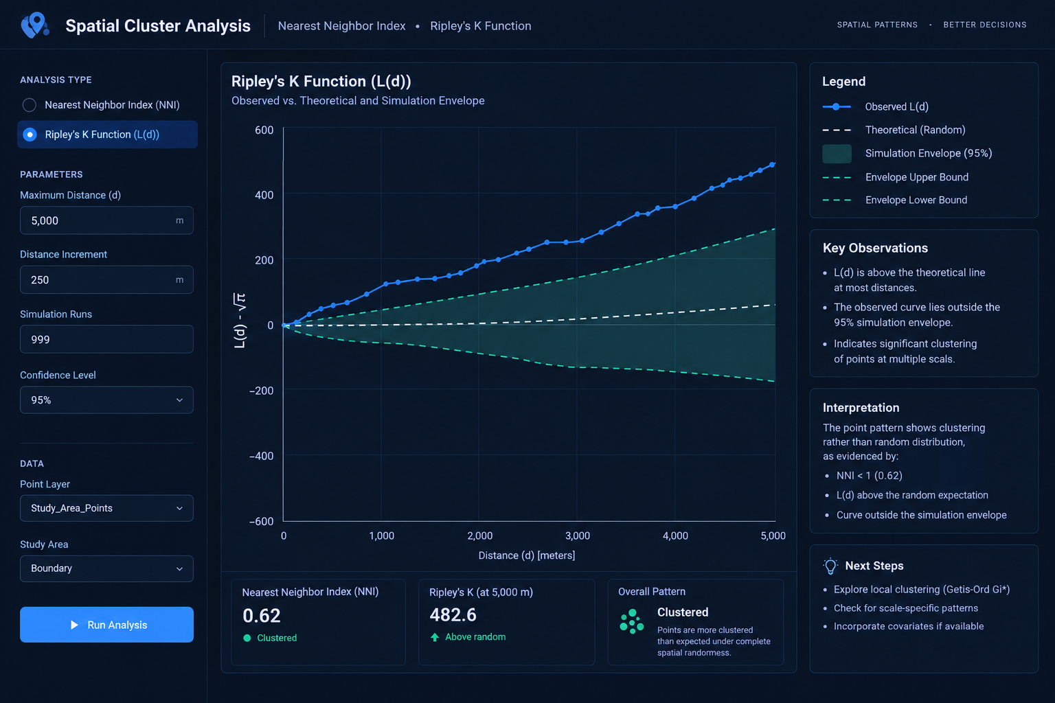
Point Pattern Analysis: Nearest Neighbor Index NNI vs Ripley’s K Function

 

1. Introduction: Understanding Point Pattern Analysis in GIS

When studying spatial point distributions, comparing tools like the Nearest Neighbor Index vs Ripley’s K Function is critical for understanding whether your data is clustered or dispersed. Imagine mapping 500 crime incidents across a city. Some incidents appear concentrated around the central business district, while others are scattered throughout residential neighborhoods. Are these patterns statistically clustered, randomly distributed, or more regularly spaced than we would expect by chance?

Point pattern analysis provides statistical methods for answering these questions by examining the geographical arrangement of point features.

It is widely used in ecology, criminology, public health, urban planning, and retail location analysis. Typical applications include mapping tree species, disease cases, accident locations, shops, and environmental sampling points.

Three general spatial patterns are commonly investigated:

• Clustered: Points occur closer together or in groups more frequently than expected under the selected random model.
• Random: The observed pattern is consistent with the selected model of spatial randomness.
• Dispersed: Points tend to be more widely separated than expected under the random model.

Visualizing the three patterns

CLUSTERED             RANDOM              DISPERSED

• •                   •       •           •      •
 •••          •             •                  •
•• •                 •   •           •
       •         •           •              •      •
• • •              •      •                       •

These diagrams are illustrative. Statistical testing is required to determine whether an observed pattern differs significantly from the chosen random baseline.

Two important methods are the Average Nearest Neighbor Index (ANN or NNI) and Ripley’s K Function. Both investigate spatial clustering, but they answer different questions.

The Nearest Neighbor Index summarizes the average distance between points and their closest neighbors at a single overall scale. Ripley’s K Function examines how the spatial pattern changes across a range of distances.

Understanding this distinction helps GIS analysts choose the appropriate method for their research question.

2. Average Nearest Neighbor Index (ANN/NNI)

2.1 What Is the Nearest Neighbor Index?

The Average Nearest Neighbor Index (NNI) compares the observed average distance between each point and its nearest other point with the average distance expected under complete spatial randomness.

In simpler terms, the method asks:

Are points generally closer together or farther apart than we would expect if their locations were random within the study area?

For example, a researcher mapping retail outlets could use NNI to determine whether stores are more closely spaced than expected or tend to be distributed regularly across a city.

2.2 How NNI Works

The calculation involves four main steps.

Step 1: Identify the nearest neighbor.

For every point, calculate the straight-line distance to its closest other point.

Step 2: Calculate the observed mean distance.

Add all nearest-neighbor distances and divide by the number of points.

Step 3: Calculate the expected mean distance.

Estimate the mean nearest-neighbor distance expected under a random distribution, using the number of points and the area of the study region.

Step 4: Calculate the index.

The NNI is the ratio of the observed mean distance to the expected mean distance:

[
NNI=\frac{\bar{d}{observed}}{\bar{d}{expected}}
]

For a two-dimensional homogeneous Poisson model, the expected mean nearest-neighbor distance is conventionally expressed as:

[
\bar{d}_{expected}=\frac{1}{2\sqrt{\lambda}}
]

Where:

[
\lambda=\frac{n}{A}
]

Here, (n) is the number of points and (A) is the study-area size.

The index compares the observed spacing with the expected spacing under this random model.

2.3 Interpreting NNI Results

NNI value	General interpretation	Spatial pattern
Less than 1	Points are closer together than expected	Clustered tendency
Approximately 1	Average spacing is consistent with the random baseline	Random-like tendency
Greater than 1	Points are farther apart than expected	Dispersed tendency

For example, suppose a university researcher maps 200 reported theft incidents within a defined urban study area.

The analysis produces an NNI of 0.65. This means the observed average nearest-neighbor distance is 65% of the expected distance under the specified random model.

The result suggests a clustered tendency, but the index alone does not establish whether the pattern is statistically significant. The researcher must also examine the associated test statistic and p-value.

Conversely, an NNI of 1.30 indicates that the observed average nearest-neighbor distance is 30% greater than expected, suggesting a dispersed tendency.

Important: An NNI near 1 does not prove that the entire point pattern is random. Different patterns can share a similar average nearest-neighbor distance.

2.4 Average Nearest Neighbor in ArcGIS Pro

ArcGIS Pro includes an Average Nearest Neighbor tool in its Spatial Statistics toolbox. It reports the observed mean distance, expected mean distance, nearest-neighbor index, z-score, and p-value. These outputs help distinguish the direction of a pattern from the statistical evidence supporting it. See the official ArcGIS Pro documentation.

A typical workflow is:

1. Prepare a point feature class containing the locations being analyzed.
2. Define a suitable study area and calculate its area correctly.
3. Ensure distance units are appropriate for the analysis.
4. Open Geoprocessing → Average Nearest Neighbor.
5. Select the input point features and distance method.
6. Supply the study-area size when needed by the tool.
7. Run the analysis and record the NNI, z-score, and p-value.

Use a projected coordinate system suitable for measuring the distances involved. Also, use the same defensible study boundary when comparing results between point datasets because changing the area can affect the expected mean distance and statistical significance.

2.5 Strengths of NNI

NNI is particularly valuable when you need a simple, interpretable summary of an overall point pattern.

Its strengths include:

• Simplicity: The index is straightforward to calculate and explain.
• Ease of interpretation: Values below and above 1 communicate the direction of the observed spacing pattern.
• Efficient analysis: It is useful for a quick assessment of whether a point distribution tends toward clustering or dispersion.
• Software accessibility: It is available directly in ArcGIS Pro and other spatial-statistics environments.

2.6 Limitations of NNI

Despite its simplicity, NNI has important limitations.

It summarizes only one nearest-neighbor scale. Because it considers only the closest neighbor to each point, it can miss patterns that appear at larger distances.

For example, trees may be regularly spaced within individual groves, while the groves themselves are clustered across a forest. NNI may fail to describe this two-level pattern adequately.

It is sensitive to the study-area boundary. The selected area affects the expected mean distance, z-score, and p-value. An arbitrary study boundary can therefore change the results.

It does not identify where clusters occur. A global NNI may indicate an overall clustered pattern but does not provide a distance-by-distance description or identify particular cluster locations.

It depends on the random reference model. A point pattern affected by strong environmental gradients or uneven population density may appear clustered relative to homogeneous randomness even when the pattern is explained by the underlying spatial variation.

Consequently, NNI is best treated as an overall summary, not a complete description of every spatial structure in the dataset.

3. Ripley’s K Function: Multi-Distance Spatial Analysis

3.1 What Is Ripley’s K Function?

Ripley’s K Function is a spatial point pattern analysis technique that examines how the number of neighboring points changes as the search distance increases.

Instead of considering only the closest neighbor, it counts other points within a specified distance of each point.

The analysis repeats this calculation across multiple distances, allowing the researcher to identify the scales at which clustering or dispersion may occur.

This makes Ripley’s K useful when the research question concerns the scale of a spatial pattern, rather than simply its overall direction.

3.2 How Ripley’s K Works

Imagine a researcher mapping tree locations in a forest. The goal is to determine whether trees cluster within short distances, at intermediate distances, or across wider sections of the forest.

Ripley’s K expands the neighborhood around each point using progressively larger distances.

Distance d1             Distance d2             Distance d3

    ______                 ___________             ______________
   /  •   \               /           \           /              \
  | •  ●  • |             |  •    •    |         |  •       •     |
   \______/               |     ●     |         |       ●         |
                          |  •     •  |         | •          •    |
                           \_________/           \________________/

 ● = focal point
 • = neighboring points

The circles are conceptual. In practice, the analysis counts neighbors within each specified distance around all points and summarizes the pattern statistically.

The process can be understood in four steps.

1. Select a series of analysis distances.
2. Count neighboring points within each distance.
3. Compare the observed neighbor counts with those expected under spatial randomness.
4. Examine how the result changes across the series of distances.

At short distances, the analysis may reveal small-scale clusters. At larger distances, it may reveal broader groupings or an overall dispersed tendency.

3.3 Understanding the K Function Formula

Ripley’s K Function is commonly expressed as:

[
K(d)=\frac{1}{\lambda}
E[\text{number of other points within distance }d]
]

Where:

• (K(d)) is the K function at distance (d).
• (\lambda) is the average point intensity, expressed as points per unit area.
• (E[\cdot]) denotes the expected number of neighboring points under the spatial process being studied.
• (d) is the specified search distance.

Under complete spatial randomness in a homogeneous two-dimensional Poisson process, the theoretical K function is:

[
K(d)=\pi d^2
]

The equation describes the expected pattern when points occur independently and uniformly throughout the study region.

Because K increases approximately with the square of distance under this reference model, its values can be difficult to interpret directly. A common solution is to apply a square-root transformation.

3.4 The L(d) Transformation

The transformed function is often expressed as:

[
L(d)=\sqrt{\frac{K(d)}{\pi}}
]

Under complete spatial randomness, the expected theoretical relationship becomes:

[
L(d)=d
]

This produces a more intuitive comparison between the observed spatial pattern and the random reference line.

Some software displays (L(d)) against the distance (d), while other implementations display the centered transformation (L(d)-d), for which the theoretical reference under complete spatial randomness is zero. Always inspect the software’s output definition before interpreting its graph.

3.5 Interpreting the L(d) Curve

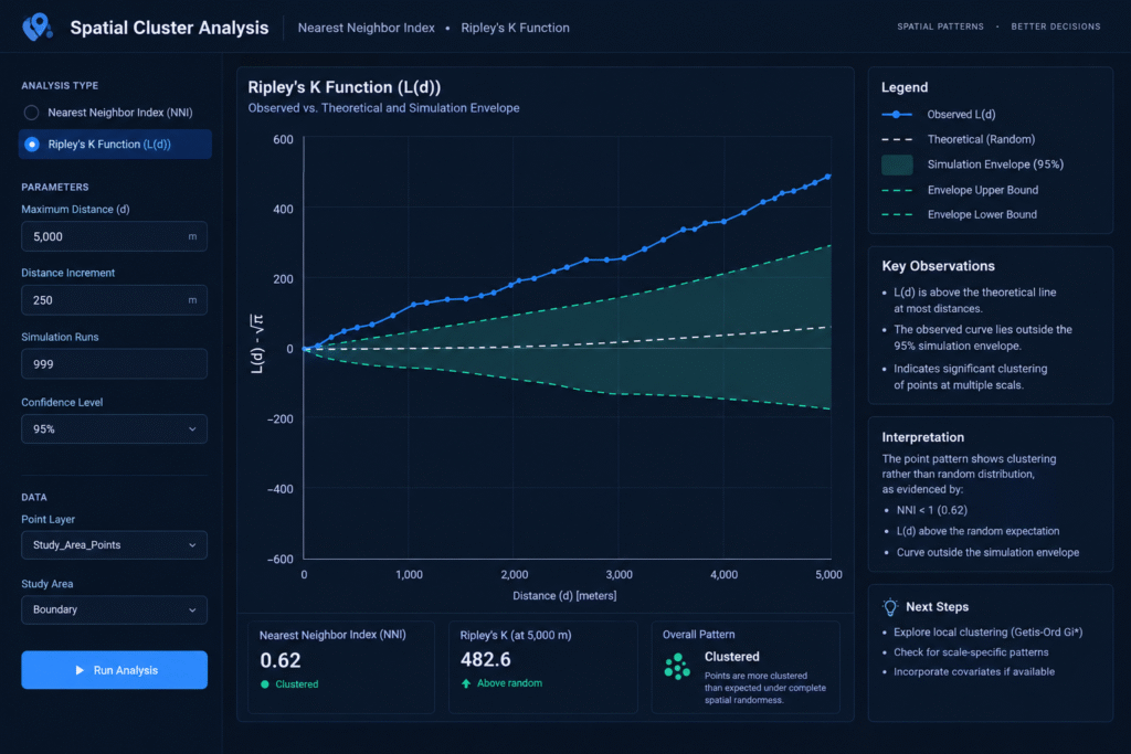
The L(d) curve shows how the observed point pattern compares with the expected random pattern as distance increases.

Curve behavior	Interpretation relative to the random reference
Observed L(d) above the expected line	More neighbors than expected; clustering tendency
Observed L(d) close to the expected line	Pattern broadly consistent with the random baseline at that distance
Observed L(d) below the expected line	Fewer neighbors than expected; dispersion tendency

For example, suppose a study of tree locations produces an observed L(d) curve that is above the expected line at distances between 10 and 40 metres, but falls below the line at distances between 100 and 150 metres.

This suggests clustering at short to intermediate distances and a dispersed tendency at larger distances, relative to the chosen reference process.

Such a pattern could arise when trees occur in small groups that are regularly spaced across the wider landscape. The interpretation would require examination of the ecology and the statistical uncertainty, rather than assuming a specific cause from the curve alone.

3.6 Why Distance Matters

One of Ripley’s K’s most important advantages is that it reveals changes in the spatial pattern across multiple distances.

Consider a retail-location dataset:

• At 100 metres, stores may be clustered around individual transport stops.
• At 1 kilometre, several commercial centers may become apparent.
• At 5 kilometres, the distribution may appear dispersed because the centers are spaced apart.

A single overall NNI cannot fully communicate these scale-dependent changes.

Ripley’s K can therefore provide more detailed insight into the spatial organization of features.

3.7 Statistical Significance and Simulation Envelopes

An observed curve lying above the expected line does not automatically demonstrate statistically significant clustering.

A common approach is to generate simulated point patterns under the chosen null model and calculate the corresponding K or L curves. These simulations create a confidence or simulation envelope.

• Where the observed curve exceeds the upper envelope, this provides evidence of more clustering than expected under the specified simulation model.
• Where the observed curve falls below the lower envelope, this provides evidence of greater dispersion than expected.
• Where the curve remains within the envelope, the analysis has not established a departure from that null model at those distances.

For global inference across the entire range of distances, a suitable global envelope procedure is preferable to relying solely on separate pointwise envelopes at each distance. Examining many distances introduces a multiple-testing concern.

ArcGIS Pro’s Multi-Distance Spatial Cluster Analysis (Ripley’s K Function) tool evaluates clustering and dispersion over a range of distances and can generate simulation-based envelopes. It also provides a documented L(d) transformation for which the expected random value equals the distance. See the ArcGIS Pro tool documentation.

3.8 Strengths of Ripley’s K Function

Ripley’s K offers several advantages for detailed point pattern investigations.

• Multiple spatial scales: It evaluates the point pattern at multiple distances instead of relying on one nearest-neighbor measurement.
• Detection of scale-dependent patterns: It can reveal clustering at short distances and dispersion at longer distances.
• Detailed interpretation: Its curve provides more information about how spatial organization changes with distance.
• Flexible applications: It is useful for ecology, urban analysis, epidemiology, and other point-based research.

3.9 Limitations of Ripley’s K Function

Ripley’s K is more informative across scales, but it also presents additional challenges.

Edge effects: Points near the boundary may have neighbors outside the observation window that were not recorded. Without appropriate correction, the analysis can underestimate neighboring points, particularly at larger distances.

Choice of study region: The boundary affects both the estimated K function and the interpretation of the reference model.

Computational demands: The analysis often involves pairwise distance calculations at multiple distance bands, which can be costly for very large datasets.

Interpretation: The curve requires more statistical knowledge than a single NNI value. Analysts must understand the reference line, simulation envelope, and the distance range being investigated.

Inhomogeneous intensity: If locations naturally occur more frequently in certain parts of the study area, homogeneous complete spatial randomness may be an unsuitable reference. An inhomogeneous K-function or another appropriate null model may be required.

Edge correction and null-model selection are therefore important parts of a defensible multi-distance analysis. See Haase’s review of Ripley’s K and edge-correction methods.

4. NNI vs Ripley’s K: Which Method Should You Use?

The choice depends primarily on the research question and the level of detail required.

4.1 Choose NNI for a Single Overall Summary

The Average Nearest Neighbor Index is appropriate when you need to characterize the overall nearest-neighbor spacing of a point dataset.

Typical examples include:

• Determining whether store locations are generally closer together than expected.
• Investigating the overall spacing of individual tree locations.
• Assessing whether reported incidents tend toward clustering or dispersion.
• Comparing datasets using the same study area and compatible assumptions.

NNI is particularly useful in introductory spatial statistics because it connects an intuitive distance measure to a statistical reference model.

4.2 Choose Ripley’s K for Multi-Distance Investigation

Ripley’s K is appropriate when your research asks how point clustering or dispersion changes across distances.

Typical examples include:

• Identifying the distance ranges associated with tree clustering.
• Examining whether disease cases cluster at local or broader spatial scales.
• Investigating the spacing of retail centers and nearby stores.
• Evaluating whether crime incidents show different patterns at neighborhood and district scales.

If understanding where the pattern changes with distance is central to the project, Ripley’s K is usually more informative.

4.3 Summary Comparison Matrix

Feature	Average Nearest Neighbor Index	Ripley’s K Function
Primary question	Are nearest-neighbor distances shorter or longer than expected?	How does spatial clustering change across distances?
Distance scale	Single overall nearest-neighbor measure	Multiple specified distances
Main output	NNI, observed distance, expected distance, z-score, and p-value	K or L(d) curve, expected reference, and optional simulation envelopes
Cluster detection	Overall clustering tendency	Clustering at different spatial scales
Dispersion detection	Overall dispersed tendency	Dispersion across specified spatial scales
Edge effects	Sensitive to the study-area size and boundary assumptions	Edge correction is particularly important for multi-distance estimation
Statistical interpretation	Relatively straightforward	Requires interpretation of curves and simulation envelopes
GIS tool	Average Nearest Neighbor in ArcGIS Pro	Multi-Distance Spatial Cluster Analysis in ArcGIS Pro
Main limitation	Can conceal patterns occurring at different spatial scales	More complex and sensitive to distance settings and the null model
Best use	Initial overall point-pattern summary	Detailed analysis of scale-dependent spatial structure

5. Practical Decision Framework

Use the following sequence when selecting a method for a university project.

Question 1: Do you need one overall measure of nearest-neighbor spacing?

Choose NNI if your main objective is to summarize the average nearest-neighbor pattern.

Question 2: Does the research require identifying the distances at which clustering occurs?

Choose Ripley’s K if the study needs multi-distance spatial analysis.

Question 3: Does the point intensity vary across the study region?

Investigate whether the selected random reference model is appropriate. For example, retail stores are often concentrated where people live or travel. A homogeneous random model could suggest clustering simply because the population itself is unevenly distributed.

Question 4: Are you comparing patterns from separate datasets?

Keep the study area, spatial scale, distance definitions, and null-model assumptions consistent where possible. Differences in geographic extent or point density can otherwise complicate comparisons.

Question 5: Is statistical significance part of the research question?

Report the relevant test results for NNI or use an appropriate simulation-envelope procedure for Ripley’s K. Do not infer significance simply because a curve lies above or below the theoretical reference.

Can You Use Both Methods?

Yes. In fact, they can complement one another.

For example, NNI can provide a concise initial assessment of the overall nearest-neighbor pattern. Ripley’s K can then investigate whether that pattern changes between short, intermediate, and longer distances.

If both methods provide similar overall evidence, the findings reinforce one another at a broad descriptive level. If their conclusions differ, that may indicate scale-dependent organization or differences in what the two statistics measure.

The discrepancy is not necessarily an error: NNI and Ripley’s K summarize different properties of a point pattern.

6. Summary Checklist for University Projects

Before submitting a point pattern analysis, use the following checklist.

• Define the research question: Clarify whether you are investigating overall nearest-neighbor spacing or spatial structure at multiple scales.

• Prepare the point dataset: Remove accidental duplicates, investigate missing coordinates, and confirm that each point represents a valid observation.

• Select an appropriate coordinate system: Use suitable projected coordinates when distances are calculated in linear units.

• Define the observation window: Explain how the study-area boundary was chosen and how it relates to the data collection process.

• Choose the method: Use NNI for the overall nearest-neighbor index or Ripley’s K for multi-distance pattern analysis.

• Specify the null model: Explain what randomness means for the study and assess whether homogeneous complete spatial randomness is suitable.

• Address boundary effects: Evaluate the study-area sensitivity of NNI and apply suitable edge correction for Ripley’s K.

• Report statistical evidence: Include the NNI, z-score, and p-value where appropriate, or interpret the K/L curve alongside its simulation envelope.

• Interpret the spatial process carefully: Distinguish a statistical clustering pattern from an explanation of its cause.

• Document the workflow: Record the software, parameters, study boundary, distance range, and other settings required to reproduce the results.

7. Conclusion

The Nearest Neighbor Index vs Ripley’s K Function GIS comparison highlights an essential principle in spatial statistics: different methods reveal different properties of geographical patterns.

The Average Nearest Neighbor Index compares the observed mean distance between each point and its closest neighbor with the expected distance under a random model. Its simplicity makes it effective for an initial, overall assessment of clustering and dispersion.

Ripley’s K Function examines how the number of neighboring points changes across multiple distances. By interpreting the transformed L(d) curve against the expected random reference and suitable simulation envelopes, analysts can investigate the spatial scales at which clustering or dispersion occurs.

For your GIS project, choose NNI when the primary question concerns overall nearest-neighbor spacing. Choose Ripley’s K when the spatial process may change with distance and the study requires multi-scale evidence.

Above all, remember that a point pattern is not simply clustered or dispersed in every possible sense. Its appearance depends on the distance scale, the geographical observation window, and the random process used as a reference. A reliable spatial analysis makes those assumptions explicit before drawing conclusions.