Buffer Analysis vs. Service Area Analysis: Which Proximity Tool Should You Use?

Introduction: Understanding Proximity Analysis in GIS

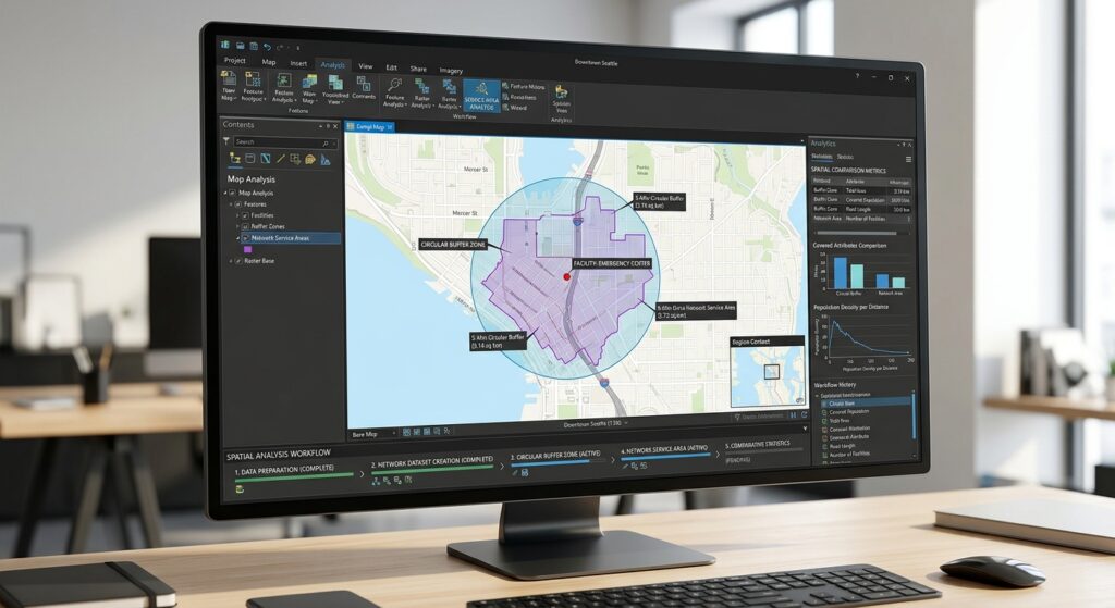
Buffer Analysis vs Service Area Analysis is one of the most important comparisons when examining proximity and accessibility in Geographic Information Systems (GIS). . It helps researchers, planners, and decision-makers understand how locations relate to nearby features, whether they are examining houses near rivers, customers near retail stores, or communities within reach of emergency services.

Two common proximity mapping tools are Buffer Analysis and Service Area Analysis. Although they may appear to answer similar questions, they measure proximity in fundamentally different ways.

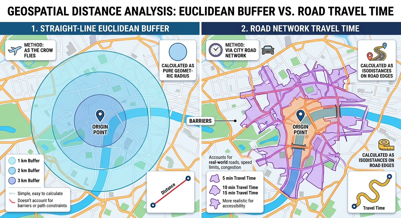
Buffer Analysis creates a zone around a geographic feature based on a specified distance. A conventional Euclidean buffer around a point produces a circle representing locations within a straight-line distance of that point.

Service Area Analysis identifies locations that can be reached from a facility through a transportation network within a specified travel distance or time. Instead of assuming movement in every direction, it accounts for the connectivity and characteristics of the network.

Consider a hospital located in a densely populated urban area. A 5-kilometer buffer can identify locations within 5 kilometers in straight-line distance. However, some residents inside that circle may need to travel much farther by road because of rivers, highways, restricted crossings, or disconnected streets. Other residents outside the circle may still be able to reach the hospital within a practical travel time.

This distinction is central to understanding Buffer Analysis vs Service Area Analysis GIS.

Neither method is universally superior. The appropriate choice depends on whether your research concerns geographic distance from a feature or accessibility through a transportation network.

1. Buffer Analysis: Measuring Straight-Line Proximity

1.1 What is Buffer Analysis?

Buffer Analysis creates polygons around point, line, or polygon features using a specified distance.

For example, a GIS analyst might create:

• A 500-meter buffer around a river.
• A 1-kilometer buffer around a school.
• A 100-meter buffer around a pipeline.
• A 200-meter buffer around a wetland boundary.

The buffer identifies the geographic zone within the selected distance, subject to the chosen measurement method and input geometry.

For a point feature, the basic Euclidean buffer is represented mathematically as:

[
B_r(p)={x(x,p)\leq r}
]

Where:

• (B_r(p)) represents the buffer around point (p).
• (d(x,p)) is the straight-line distance between location (x) and point (p).
• (r) is the specified buffer radius.

For a point with a 1,000-meter buffer, all locations within 1,000 meters in the selected planar measurement system fall within the buffer.

1.2 Euclidean buffers

Euclidean buffers calculate straight-line distances in a two-dimensional coordinate plane.

For two points with coordinates ((x_1,y_1)) and ((x_2,y_2)), the Euclidean distance is:

[
d=\sqrt{(x_2-x_1)^2+(y_2-y_1)^2}
]

A Euclidean buffer is particularly useful when working within a suitable projected coordinate system covering a relatively small study area.

For example, imagine a school in a town. You want to identify residential buildings within 1 kilometer of the school, without considering how residents travel.

A Euclidean buffer provides a straightforward way to identify those buildings.

However, the resulting zone does not establish that each building is reachable by road within 1 kilometer. It only describes straight-line proximity.

Important: Use an appropriate projected coordinate system with suitable distance properties. Calculating planar distances directly from longitude and latitude values expressed in degrees can produce misleading measurements.

1.3 Geodesic buffers

Geodesic buffers account for the curvature of the Earth rather than treating the study area as a flat coordinate plane.

They are useful when features cover large geographic regions, span multiple projection zones, or are represented in coordinate systems that significantly distort distances.

Both Euclidean and geodesic buffers measure geographic proximity rather than travel through a road network. A geodesic buffer may improve the accuracy of the distance measurement, but it does not account for roads, traffic, rivers that obstruct movement, or one-way streets.

For local environmental studies, a suitable projected CRS and planar buffer may be sufficient. For extensive or global datasets, geodesic methods may be more appropriate.

Esri explains these distinctions in its Buffer analysis documentation.

1.4 Advantages of Buffer Analysis

Buffer Analysis offers several practical advantages.

Simple implementation: Most desktop GIS applications provide a standard Buffer tool, making the workflow accessible to beginners.

Efficient processing: Standard buffer operations are generally computationally inexpensive compared with detailed network-based accessibility analysis, although processing time depends on the feature count, geometry complexity, and implementation.

Flexible geometry: Buffers can be created around points, lines, and polygons, with options for multiple distances and dissolving overlapping zones.

Broad applicability: Buffers support environmental assessment, infrastructure planning, land-use regulation, and many forms of spatial screening.

Clear interpretation: A buffer distance communicates a direct geographic threshold that can be measured and mapped.

1.5 Limitations of Buffer Analysis

Despite its simplicity, a buffer can be inappropriate when the research question concerns movement or practical accessibility.

For example, a residential property may be only 800 meters from a hospital in straight-line distance but 2.5 kilometers away by road.

A circular buffer would classify the property as being within a 1-kilometer proximity zone, even though the road route exceeds that distance.

Other limitations include:

• Failure to represent road connectivity.
• No inherent modeling of one-way streets or restricted access.
• No travel-time calculation unless additional methods are applied.
• Potential distortion if the distance method or CRS is unsuitable.
• No direct consideration of barriers to movement.

These limitations do not make buffers inaccurate for their intended purpose. They indicate that the method answers a different question from network accessibility analysis.

1.6 Appropriate use cases for Buffer Analysis

Buffer Analysis is generally appropriate when the research concerns a geographic zone around a feature rather than how people or vehicles travel.

Scenario	Example analysis	Why a buffer is suitable
Environmental protection	A 30-meter zone around a riverbank	Identifies locations within a defined geographic setback
Noise assessment	A 500-meter zone around an industrial facility	Screens properties near a potential noise source
Infrastructure planning	A 100-meter zone around a pipeline	Identifies nearby land parcels or assets
Land-use regulation	A setback around a protected wetland	Supports geographic restriction mapping
School proximity	Buildings within 1 kilometer of a school	Measures straight-line proximity
Hazard screening	Properties within a defined radius of a potential hazard	Identifies features within a geographic threshold

For a river buffer, remember to define whether the setback is measured from the mapped bank, the river centerline, or another legally or scientifically specified boundary. This distinction affects the result.

2. Service Area Analysis: Measuring Network Accessibility

2.1 What is Service Area Analysis?

Service Area Analysis determines the locations or network segments reachable from a facility within a specified travel cost.

The cost may represent:

• Travel distance.
• Travel time.
• Another defined network impedance, such as generalized travel cost.

Unlike a conventional buffer, service area analysis follows a network of connected edges, such as streets or pedestrian paths.

It can therefore represent the difference between geographic closeness and practical accessibility.

For example, an emergency response service may need to identify all roads reachable within five minutes of a fire station under a specified travel model.

A circular buffer around the station cannot directly determine this coverage because it does not follow the road network.

Esri defines a network service area as the region encompassing the streets reachable within a specified distance or travel time from a facility. See the ArcGIS Network Analyst solver documentation.

2.2 How road-network analysis works

A routable road network can be represented as a graph consisting of:

• Nodes: Junctions, intersections, and connected network locations.
• Edges: Road or path segments connecting those nodes.
• Impedance: A cost assigned to traversing network edges.
• Restrictions: Rules that limit travel, such as prohibited turns or one-way streets.

A network solver evaluates the routes from a facility through connected edges while respecting the selected travel settings.

For a distance-based analysis, a route’s cost might be the total length of the traversed edges:

[
D(P)=\sum_{i=1}^{n}l_i
]

Where:

• (D(P)) is the distance along route (P).
• (l_i) is the length of the (i)-th traversed network edge.
• (n) is the number of traversed edges.

For a time-based analysis, the total travel time may be represented as:

[
T(P)=\sum_{i=1}^{n}\frac{l_i}{v_i}
]

Where (v_i) represents the modeled travel speed on edge (i).

This simplified time equation assumes constant speed within each edge and omits additional effects unless they are incorporated into the network cost model. Real routing services may use more sophisticated travel-time attributes, restrictions, and traffic models.

The service area includes network locations reachable without exceeding the specified cost threshold.

2.3 Travel time versus travel distance

Service areas can be defined using either distance or time, but the two are not interchangeable.

A 3-kilometer network service area includes places reachable within 3 kilometers of network travel distance. A 10-minute service area includes places reachable within 10 minutes according to the selected travel-time model.

The time-based result may vary with:

• Road classification.
• Mode of travel.
• Speed assumptions.
• One-way restrictions.
• Turn restrictions.
• Traffic conditions, where supported.
• Departure or arrival time, where supported.

For example, a 10-minute driving service area may differ considerably from a 10-minute walking service area around the same facility.

2.4 Understanding service area polygons

A network analysis can produce reachable road segments, boundary locations, and service area polygons.

The polygons summarize the network area reachable within the specified cost. They are often useful for presentation and overlay analysis, but they should not be interpreted as proof that every location inside the polygon is directly accessible from a road.

The extent and shape of the polygons depend on the network, the cost threshold, polygon generation settings, and how the road network is represented.

When evaluating population coverage, for instance, consider whether residents are connected to the road or pedestrian network and whether the polygon appropriately represents access at the scale of the study.

2.5 Advantages of Service Area Analysis

More realistic network accessibility: The analysis follows connected roads or paths rather than assuming movement is possible in every direction.

Travel-time estimation: It can identify areas reachable within specified driving, walking, or other supported travel times.

Network restrictions: A suitable network dataset can incorporate one-way rules, turn restrictions, and other impedances.

Operational planning: It supports emergency response planning, retail catchment studies, healthcare accessibility, and transport planning.

Multiple service thresholds: Analysts can compare nested or separate service areas, such as 5-, 10-, and 15-minute drive-time coverage.

2.6 Limitations of Service Area Analysis

Service Area Analysis provides richer accessibility modeling, but its results depend heavily on the quality and assumptions of the network.

Important limitations include:

• Requires a suitable routable network or routing service.
• May need additional software extensions, permissions, or service credits, depending on the platform.
• Usually requires more processing and configuration than a simple buffer.
• Can produce misleading results if roads are missing or connectivity is incorrect.
• Travel-time estimates may be unreliable if speed assumptions and traffic conditions do not reflect actual movement.
• May not represent off-network movement, informal paths, private access restrictions, or real-world barriers unless modeled.

A high-quality network analysis should therefore document the network source, travel mode, impedance settings, restrictions, cutoff values, and any time-dependent parameters.

2.7 Appropriate use cases for Service Area Analysis

Scenario	Example analysis	Why a service area is suitable
Emergency response	Roads reachable within 5 minutes of a fire station	Represents network travel time
Healthcare access	Residential areas within a 15-minute drive of a hospital	Models road accessibility
Retail planning	Customers within a 10-minute drive of a supermarket	Better represents a potential driving catchment
Public transport	Areas reachable within a defined walking or transit cost, if supported by the model	Incorporates the relevant network and travel mode
Delivery operations	Locations reachable within a 20-minute delivery route cost	Uses modeled network movement
Public service planning	Communities reachable within a specified walking distance of a facility	Can represent pedestrian-network accessibility

For retail and healthcare studies, service areas are usually more informative than circles when access occurs primarily through a road network. However, demographic data, facility capacity, travel mode, and other factors may still be needed to evaluate actual service use or unmet demand.

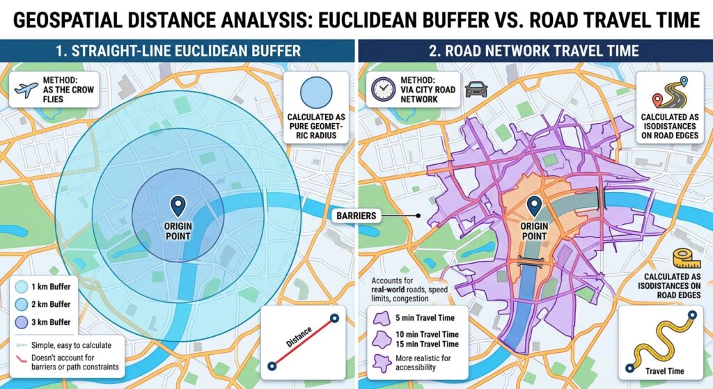
3. Buffer Analysis vs. Service Area Analysis: Comparison Matrix

The following matrix summarizes the major differences between the two methods.

Criterion	Buffer Analysis	Service Area Analysis
Distance type	Straight-line Euclidean or geodesic distance	Network travel distance, time, or another impedance
Network requirement	No road network required	Requires a suitable network or routing service
Computational speed	Usually faster and simpler	Often more computationally demanding
Geographic shape	Commonly circular around points, with other shapes for lines and polygons	Irregular shape following reachable network paths
Real-world accessibility	Does not directly model travel along routes	Models network-based reachability subject to network quality
Travel time	Not measured by a standard distance buffer	Supported when the network has suitable travel-time costs
Road restrictions	Not represented inherently	Can be modeled if the network contains the relevant restrictions
Environmental zones	Well suited to fixed-distance geographic restrictions	Usually unnecessary unless access or movement along a network is the research focus
Data preparation	Geometry and coordinate system checks	Geometry, coordinate system, network topology, connectivity, and cost-model checks
Best use case	Setbacks, environmental zones, hazard screening, and straight-line proximity	Emergency response, realistic travel coverage, healthcare accessibility, and retail catchments

The central distinction

A buffer asks:

“Which locations are within this geographic distance of the feature?”

A service area asks:

“Which locations can be reached through this network within the specified travel cost?”

Those questions may produce different spatial results even when the nominal distance values are identical.

4. Scenario-Based Examples

Scenario A: Protecting a river corridor

A researcher wants to identify land parcels within 50 meters of a river.

Recommended method: Buffer Analysis.

The research concerns a fixed geographic setback from the mapped riverbank or another defined boundary. A buffer can create the relevant corridor without requiring a road network.

The researcher should establish the correct river geometry, horizontal measurement method, and reference boundary. If regulations specify that the distance should be measured from the bank, buffering a river centerline may not satisfy the requirement.

A service area would be inappropriate unless the objective concerned access along paths or roads near the river rather than physical proximity.

Scenario B: Evaluating emergency response coverage

A county government wants to determine which roads are reachable within eight minutes of each fire station.

Recommended method: Service Area Analysis.

The analysis needs a routable street network and an eight-minute travel-time threshold.

A circular eight-minute buffer has no direct travel-time interpretation because distance traveled in eight minutes varies according to the route, speed, and network restrictions.

The service area should document the driving mode, time assumptions, network source, cutoff, and any available traffic settings. The output can then be compared with incident locations or population data to identify potential coverage gaps.

Scenario C: Assessing school accessibility

A planning team wants to identify residential locations within 1 kilometer of a primary school.

The correct method depends on the meaning of “within 1 kilometer.”

If the objective is simply to measure geographic proximity, a 1-kilometer buffer is appropriate.

If the objective is to estimate which residential locations can reach the school by walking within 1 kilometer along available pedestrian routes, use a suitable pedestrian-network service area.

If pedestrian paths, road crossings, informal routes, or barriers are missing from the network, the service area may still underestimate or overestimate real accessibility. The network needs to represent the travel mode studied.

Scenario D: Selecting a retail location

A company wants to understand which neighborhoods could be reached within a 12-minute drive of a proposed store.

Recommended method: Service Area Analysis.

A 12-minute drive-time service area more closely represents the intended catchment than a circular buffer, provided that the network and travel-time assumptions are suitable.

However, a service area alone does not predict how many residents will actually shop at the store. Demand, competing retailers, purchasing behavior, road congestion, and other influences may require additional analysis.

Scenario E: Screening properties near an industrial facility

An environmental analyst wants to identify buildings within 500 meters of an industrial site for a preliminary proximity assessment.

Recommended method: Buffer Analysis.

A geographic buffer can identify nearby buildings for screening. If the actual objective concerns air pollution, noise exposure, or contaminant dispersion, a buffer should not be treated as a substitute for an appropriate exposure model.

The distance threshold should be justified by the study design, regulations, or a defensible screening assumption.

5. Practical Software Considerations

5.1 Buffer Analysis in QGIS or ArcGIS Pro

Both QGIS and ArcGIS Pro provide buffer tools.

A typical workflow is:

1. Load the input point, line, or polygon layer.
2. Verify the coordinate reference system and measurement units.
3. Open the Buffer geoprocessing tool.
4. Specify the distance and, where relevant, the measurement method.
5. Choose whether individual buffers should remain separate or be dissolved.
6. Run the tool and inspect the output against the original features.

For a local study, use an appropriate projected coordinate system when performing planar distance operations. For large or geographically dispersed datasets, consider geodesic buffering.

5.2 Service Area Analysis in QGIS

QGIS includes network-analysis tools in the Processing Toolbox, including Service area (from layer) and Service area (from point).

A typical workflow is:

1. Prepare a connected road or path network.
2. Load the origin or facility points.
3. Open Processing Toolbox → Network analysis → Service area.
4. Choose the network and starting facilities.
5. Select the path strategy, such as shortest distance or fastest travel time.
6. Set the travel-cost threshold and relevant network settings.
7. Run the analysis and review the reachable network segments or boundary output.

The exact output and time or distance behavior depend on the selected algorithm and configuration. See the QGIS network analysis documentation.

5.3 Service Area Analysis in ArcGIS Pro

ArcGIS Pro supports service area analysis through Network Analyst.

A typical workflow is:

1. Prepare a suitable network dataset or identify an available routing service.
2. Open the Network Analyst or relevant geoprocessing workflow.
3. Create a Service Area analysis layer.
4. Add facility locations.
5. Select the travel mode and impedance, such as driving time or distance.
6. Enter the cutoffs, such as 5 and 10 minutes.
7. Configure travel direction and other relevant settings.
8. Solve the analysis and inspect the resulting network coverage.

Local network analysis requires the appropriate data and licensing. Using online routing services can introduce service limits, credit consumption, or input restrictions depending on the service and account.

Refer to Esri’s Make Service Area Analysis Layer documentation for detailed parameters.

6. Decision Matrix for GIS Students

Use this decision matrix to select an appropriate proximity tool for a research assignment or dissertation.

Research question	Recommended method	Reason
Which houses are within 100 meters of a river?	Buffer Analysis	Fixed geographic distance
Which locations are within 3 kilometers in straight-line distance of a school?	Buffer Analysis	Direct spatial proximity
Which roads can a fire engine reach within 6 minutes?	Service Area Analysis	Network-based travel time
Which customers are within a 10-minute drive of a shop?	Service Area Analysis	Travel-time catchment
Which parcels lie within a regulatory setback from a pipeline?	Buffer Analysis	Defined geographic restriction
Which communities have poor access to hospitals by road?	Service Area Analysis, usually with demand and coverage analysis	Network-based access and potential coverage gaps
Which homes are within a 2-kilometer walking route of a bus stop?	Service Area Analysis using a pedestrian network	Measures route distance rather than straight-line distance
Which buildings are near a potential noise source?	Buffer Analysis for initial screening	Geographic proximity, with further exposure modeling if needed

Three questions to ask before selecting a method

1. Does the research concern physical proximity or movement?

If it concerns distance from a feature regardless of travel routes, buffering may be sufficient. If it concerns the ability to reach a place, consider network-based analysis.

2. What does the distance threshold mean?

A 500-meter buffer measures geographic proximity. A 500-meter network service area measures travel along connected network segments. A 10-minute service area measures modeled travel time. These are not equivalent measurements.

3. Does the input data support the required assumptions?

A road network with missing links may produce unreliable service areas. A layer with an unsuitable CRS may produce inaccurate planar buffers. The method and the data must be appropriate for the same research objective.

Conclusion

Buffer Analysis and Service Area Analysis are complementary proximity mapping tools. The distinction lies in the type of distance being measured and the assumptions about how movement occurs.

Use Buffer Analysis when your objective is to identify geographic areas within a fixed distance of points, lines, or polygons. It is especially useful for environmental setbacks, infrastructure zones, hazard screening, and straight-line proximity studies.

Use Service Area Analysis when your objective is to determine the locations reachable along a road or pedestrian network within a given distance or travel time. It is especially useful for realistic travel coverage, emergency response planning, transport accessibility, and retail catchment assessment.

For GIS students, the most important lesson is to define the research question before selecting the tool. A technically correct buffer can still be inappropriate for a travel-accessibility question, while a detailed network service area may be unnecessary for a simple environmental setback.

The best proximity method is the one that matches the meaning of distance in your research, uses data that supports the required assumptions, and produces results that can be interpreted responsibly.