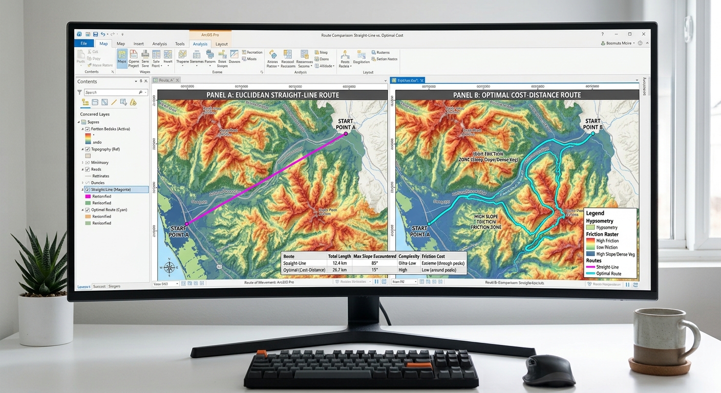
Cost-Distance & Least-Cost Path Analysis in ArcGIS Pro & QGIS

1. Introduction: What Is Least-Cost Path Analysis?

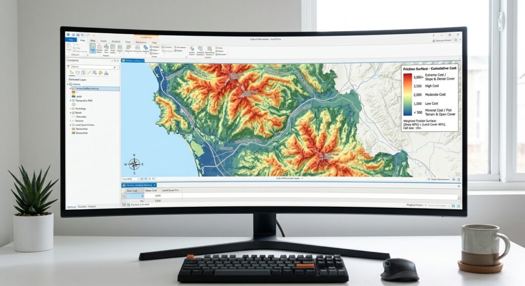
Imagine a transportation agency planning a new road between two towns. The shortest route on a map might cross steep mountains, wetlands, protected habitats, or densely developed neighborhoods. Although geographically short, that route could be expensive to construct and environmentally damaging.

Least-Cost Path Analysis (LCPA) is a GIS technique that identifies a route between locations by minimizing the cumulative cost of moving across a landscape.

Instead of considering only distance, the analysis uses a cost surface, also called a friction surface, to represent the relative difficulty, expense, or impact of traversing each raster cell.

The technique is widely used in:

• Road, pipeline, and electrical transmission-line planning.
• Wildlife movement and ecological corridor mapping.
• Hiking trails and emergency access route planning.
• Environmental impact assessment.
• Infrastructure site selection.

The central idea is straightforward: a route can be longer geographically but preferable overall because it passes through areas with lower costs.

1.1 How Does Least-Cost Path Analysis Work?

The workflow has three main analytical outputs or stages:

1. Cost surface: Represents the resistance associated with traversing each cell.
2. Cost-distance accumulation: Calculates the minimum cumulative cost from a source to every reachable cell.
3. Least-cost path: Traces the route between a destination and its least-cost source using the accumulated-cost and direction information.

The cumulative cost of a route can be represented conceptually as:

[
C(P)=\int_P c(s),ds
]

Where:

• (P) is a candidate route.
• (c(s)) represents the local traversal cost along the route.
• (ds) represents an incremental distance along the route.

In raster analysis, the integral is approximated using cell traversal costs and the distances moved between cells.

The result is the route that minimizes cumulative cost under the selected cost model, raster resolution, and movement assumptions.

Important: Least-cost path analysis does not automatically find the cheapest real-world road or pipeline. It finds the minimum-cost route according to the criteria and weights supplied by the analyst.

2. Step 1: Creating the Cost or Friction Surface

The cost surface is the foundation of the entire analysis. If its values poorly represent the problem, the resulting route may be mathematically optimal but practically unsuitable.

For example, a road construction project may prioritize gentle slopes, open terrain, and avoidance of settlements. A wildlife corridor may prioritize suitable habitat and penalize roads, settlements, and other barriers.

The same geographical area can produce very different least-cost paths depending on the purpose of the project.

2.1 Prepare the Required Input Data

Typical input datasets include:

Input dataset	Purpose	Example source
Digital Elevation Model (DEM)	Derive slope and terrain characteristics	SRTM, Copernicus DEM
Land-cover raster	Represent the relative difficulty of traversing different surfaces	Sentinel-2 classification, national land-cover maps
Environmental constraints	Represent protected areas, wetlands, forests, and sensitive habitats	Protected-area datasets, environmental agencies
Source point	Starting location of the proposed route	Road junction, power station, water-treatment plant
Destination point	Ending location of the proposed route	Town, distribution station, industrial facility

Before analysis, make sure all input rasters have compatible:

• Coordinate reference systems.
• Cell sizes and grid alignment.
• Spatial extents.
• NoData conventions.

Use a suitable projected coordinate system when working with local or regional routes so that the raster cell dimensions represent meaningful ground distances.

The raster resolution should reflect the planning scale. A very coarse raster may overlook narrow streams, roads, or steep terrain, while a very fine raster can greatly increase processing time and memory requirements.

2.2 Reclassify Land Cover into Traversal Costs

Land-cover classes are categorical. To use them in least-cost analysis, convert them into numerical values representing relative resistance.

For an illustrative road or transmission-line planning project, a reclassification table might look like this:

Land-cover class	Example cost	Interpretation
Open or bare ground	1	Relatively easy to traverse
Grassland or cropland	2	Low relative resistance
Shrubland	4	Moderate resistance
Forest	7	Higher construction or environmental cost
Dense urban development	9	High relative cost
Wetlands	10	Very high relative cost
Prohibited area	NoData	Route cannot cross this cell

These values are hypothetical. They should be developed using the project requirements, engineering evidence, environmental assessments, and stakeholder priorities.

For wildlife corridors, the cost interpretation may differ: intact suitable habitat could receive a low cost, while roads and urban areas could receive high costs or be treated as barriers.

A high cost means an area is discouraged, not necessarily prohibited. Use NoData or another explicitly defined barrier treatment for areas that truly cannot be crossed, and verify that the chosen software handles those barriers as intended.

2.3 Calculate Slope from the DEM

Slope helps represent the influence of terrain on construction, walking, and other forms of movement.

In QGIS:

1. Open Processing Toolbox.
2. Search for Slope under GDAL raster terrain analysis.
3. Select the DEM as the input raster.
4. Set the output measurement to degrees if that option is available.
5. Run the tool to create a slope raster.

In ArcGIS Pro:

1. Open Analysis → Tools.
2. Search for Slope.
3. Select the DEM.
4. Set the measurement method and output units appropriately.
5. Run the tool.

Reclassify the slope raster according to a project-specific resistance scheme. For example:

Slope	Example cost
0–5°	1
Greater than 5–15°	3
Greater than 15–25°	7
Greater than 25°	10

These categories are illustrative rather than universal engineering standards. A pipeline, highway, wildlife path, and transmission line may have different requirements.

2.4 Combine the Criteria into One Cost Surface

If your analysis includes land cover, slope, and environmental sensitivity, combine their reclassified values into a single friction raster.

First, normalize the criteria to comparable scales. For this example, assume each cost layer uses a scale from 1 to 10.

Assign weights based on the project’s priorities:

• Land cover: 50%
• Slope: 30%
• Environmental sensitivity: 20%

The weighted cost surface is:

[
C=0.5L+0.3S+0.2E
]

Where:

• (L) is the land-cover cost.
• (S) is the slope cost.
• (E) is the environmental cost.

The weights sum to 1, making the resulting weighted score remain on the common 1–10 scale when the input values use that same range.

A different project may justify different weights. Document the reasoning behind every criterion and weight rather than selecting values solely because they produce a visually attractive route.

In QGIS

Open Processing Toolbox → Raster Calculator and enter:

0.5 * "landcover_cost@1"
+
0.3 * "slope_cost@1"
+
0.2 * "environment_cost@1"

Save the result as:

friction_surface.tif

The expression assumes all three rasters are aligned and use the same grid. Raster cells representing absolute barriers should remain NoData in the final cost surface, rather than being assigned an ordinary low cost.

In ArcGIS Pro

Open Analysis → Tools → Raster Calculator and use:

0.5 * "landcover_cost" + \
0.3 * "slope_cost" + \
0.2 * "environment_cost"

Save the output as friction_surface.tif.

Confirm that the output cell size, extent, and snap raster are consistent with the input layers. If the criteria use different resolutions, resample or align them deliberately before combining them.

Checkpoint: Display the resulting friction surface using a graduated colour ramp. Low-cost cells should correspond to areas that are relatively easy or desirable to traverse, while high-cost cells should correspond to areas that are more difficult, expensive, or damaging.

3. Step 2: Computing Cost-Distance and Backlink Rasters

Once the cost surface is ready, calculate the cumulative cost of reaching every cell from the designated source.

The processing tool also needs to produce a direction raster. Depending on the software, this is known as a back direction, movement direction, or direction-to-source raster.

It identifies the next cell along a least-cost route back toward the source and is used to reconstruct the path.

3.1 ArcGIS Pro: Distance Accumulation

Recent ArcGIS Pro workflows use Distance Accumulation, which supports weighted distance calculations and generates the rasters needed for optimal path analysis. The newer distance tools are recommended over the legacy Cost Distance workflow. See Esri’s Distance toolset overview.

Follow these steps:

1. Open Analysis → Tools.
2. Search for Distance Accumulation in the Spatial Analyst toolbox.
3. Set the source point or source features as the input source data.
4. Set friction_surface.tif as the input cost raster.
5. Specify an output distance accumulation raster, such as accumulated_cost.tif.
6. Specify an output back direction raster, such as back_direction.tif.
7. Confirm the cell size, extent, and other analysis settings.
8. Run the tool.

The output distance accumulation raster records the minimum accumulated cost from the source to each reachable cell. The back direction raster records how a path can be traced back toward the source.

If you want a straight-line route rather than a cost-weighted route, do not supply a cost raster. If slope or other directional movement factors are required, configure them appropriately rather than assuming that the cost raster accounts for every process automatically.

The Spatial Analyst extension is required for these tools.

3.2 QGIS: GRASS GIS r.cost

QGIS provides access to the GRASS GIS cost-distance algorithm through the Processing Toolbox, provided the GRASS provider is enabled.

The r.cost tool calculates cumulative traversal cost and can produce a movement direction raster. This direction raster is subsequently used to trace the least-cost path. See the official GRASS r.cost documentation.

Follow these steps:

1. Open Processing Toolbox.
2. Search for r.cost.
3. Select friction_surface.tif as the input cost raster.
4. Specify the source point or source coordinates.
5. Set the cumulative cost output to accumulated_cost.
6. Set the movement-direction output to movement_direction.
7. Define the computational region and resolution so that they match the cost surface.
8. Run the tool.

The resulting rasters record cumulative cost and the direction used to return toward the source.

A conceptual GRASS command is:

# Calculate cumulative cost from the source location.
r.cost \
  input=friction_surface \
  output=accumulated_cost \
  outdir=movement_direction \
  start_coordinates=500000,9900000

Replace the example coordinates with the source’s easting and northing in the working projected coordinate system.

QGIS may use temporary GRASS map names within its processing session. Select the corresponding layers in the Processing Toolbox rather than assuming that the example filenames already exist.

4. Step 3: Generating the Least-Cost Path

At this stage, you have:

• The friction surface.
• The accumulated cost raster.
• The back direction or movement-direction raster.
• A destination location.

The final operation traces a route from the destination back toward the least-cost source.

4.1 ArcGIS Pro: Optimal Path As Line

In ArcGIS Pro, use the Optimal Path As Line tool. It creates a polyline feature representing the least-cost route. The input destination, distance accumulation raster, and back direction raster must be compatible. See the official Optimal Path As Line documentation.

Follow these steps:

1. Open Analysis → Tools.
2. Search for Optimal Path As Line.
3. Select the destination point or destination features.
4. Set accumulated_cost.tif as the input distance accumulation raster.
5. Set back_direction.tif as the input back direction raster.
6. Specify an output line feature class, such as least_cost_route.
7. Choose the path type appropriate to the destinations.
8. Run the tool.

For a single destination, the path type should be selected according to the intended source-to-destination relationship. For multiple destinations, options such as Each Zone and Best Single have different meanings, so review the tool documentation before choosing.

The output line includes a PathCost field that records the accumulated cost of the route. This is useful for comparing alternative routes generated under the same cost model.

4.2 QGIS: Extract the Path Using GRASS r.drain

In QGIS, search the Processing Toolbox for r.drain.

The GRASS r.drain tool can trace a path through a cost surface using the movement direction raster produced by r.cost. With the cost-surface flag enabled, it follows the supplied direction information. See the official GRASS r.drain documentation.

Follow these steps:

1. Open Processing Toolbox → r.drain.
2. Set the original friction_surface raster as the input cost surface.
3. Set movement_direction as the direction raster.
4. Enable the option or flag for a cost surface (the -d flag).
5. Specify the destination point or its coordinates as the path’s starting location for tracing.
6. Set an output path raster, such as least_cost_path_raster.
7. Where available, specify the optional drain vector output, such as least_cost_route.
8. Run the tool.

The important directional detail is that r.cost calculated movement directions toward the source. Therefore, r.drain begins tracing at the destination and follows those directions back toward the source.

A conceptual GRASS command is:

# Trace from the destination back to the source.
# movement_direction was generated by r.cost.
r.drain \
  -d \
  input=friction_surface \
  direction=movement_direction \
  output=least_cost_path_raster \
  drain=least_cost_route \
  start_coordinates=510000,9895000

Use your real destination coordinates, and ensure they are expressed in the same projected coordinate system as the raster. The drain option requests a vector representation of the traced path.

If your processing interface or GRASS version uses slightly different parameter labels, inspect the available r.drain options and enable the equivalent cost-surface and direction settings.

4.3 Inspect and Validate the Route

After generating the path, load it into the map canvas and compare it with the friction surface, terrain, streams, settlements, and other constraints.

Check the following:

• Does the route begin and end at the correct locations?
• Does it pass through any prohibited cells?
• Does it appear to avoid high-cost terrain where alternatives exist?
• Is the path excessively jagged because of raster resolution?
• Are there unexpected gaps or terminations caused by NoData areas or unconnected regions?

If the path fails to reach the destination, verify that both endpoints fall within valid cost-surface cells and that there is a continuous traversable route between them.

A least-cost path is a model-derived route, not a surveyed engineering alignment. Infrastructure projects require additional ground validation, engineering design, and regulatory assessment.

5. Step 4: Comparing Euclidean Routing with Least-Cost Routing

One of the most useful outcomes of least-cost analysis is the ability to compare a straight-line route with a cost-weighted route.

Euclidean routing connects two points using the shortest straight-line distance. It does not account for surface resistance unless additional constraints are explicitly incorporated.

Least-cost routing minimizes the accumulated cost of traversing the friction surface.

Consider this simplified diagram:

EUCLIDEAN ROUTE             LEAST-COST ROUTE

S ---------------- D       S ---\       /--- D
                                 \     /
                          HIGH-COST AREA
                              (AVOIDED)

S = Source
D = Destination

The illustration is conceptual. A real least-cost route is determined by the entire raster cost surface, not simply by avoiding a single obstacle.

5.1 How the Two Routes Differ

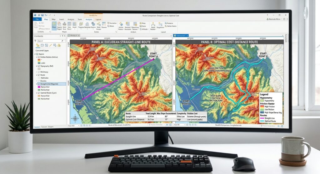
A Euclidean route may be geographically shorter but cross steep slopes, water bodies, protected habitats, or densely developed areas.

A least-cost path may follow a longer route that has a lower total impedance.

For example, the straight-line distance between a power station and a substation may be 10 kilometres, while a least-cost route follows 13 kilometres of gentler terrain. If steep slopes are assigned high costs, the longer route can still have a lower accumulated cost.

However, physical route length and accumulated cost are different quantities.

Do not compare the numerical value of a cost-distance raster directly with a distance in metres unless your cost model has been defined in compatible units. The route length can be measured separately from the resulting vector line, while the cumulative cost describes its relative suitability under the friction model.

For a fair comparison, measure both:

• Straight-line distance.
• Least-cost route length.
• Accumulated cost of the least-cost route.

Also consider whether alternative weights, raster resolutions, or barrier definitions substantially change the route.

6. Real-World Applications

6.1 Conservation Biology: Wildlife Corridors

Ecologists often need to identify potential connections between separated habitat patches.

A wildlife corridor can be modeled using a friction surface in which:

• Suitable natural habitat has low resistance.
• Fragmented habitat has higher resistance.
• Roads and built-up areas have high resistance or are modeled as barriers.
• Sensitive habitats can be assigned costs reflecting the study objectives.

The least-cost path identifies one low-cost connection between habitat areas.

For corridor planning, however, a single route may not capture the full range of possible animal movement. Consider multi-route analysis, least-cost corridor methods, or circuit-theory approaches when evaluating broader connectivity.

The selected cost values should reflect the focal species’ ecology. A route favorable to one species may not be suitable for another.

6.2 Infrastructure Planning: Roads and Pipelines

For roads, pipelines, and transmission lines, the cost surface may represent construction difficulty, land acquisition, environmental impact, or a combination of these factors.

Potential criteria include:

• Terrain slope and ruggedness.
• Land-cover type.
• Distance from settlements.
• Protected areas and wetlands.
• Existing transport access.
• Geological or flood hazards.
• Construction and maintenance costs.

Each criterion should be translated into a documented cost scale. Hard constraints must be distinguished from areas that are merely expensive or undesirable.

The resulting path can be used to compare planning alternatives, identify areas requiring detailed environmental review, and estimate the relative trade-offs among competing alignments.

For real-world engineering, the GIS route remains a preliminary alignment. Detailed surveying, hydrological analysis, geotechnical investigations, and legal constraints must also be considered.

7. Conclusion and Key Takeaways

Cost-distance and least-cost path analysis provide a systematic way to identify routes that minimize cumulative landscape resistance rather than simple geographic distance.

In ArcGIS Pro, a common modern workflow is to generate accumulated cost and back-direction rasters with Distance Accumulation, then create a line using Optimal Path As Line.

In QGIS, a comparable workflow uses the GRASS r.cost tool to compute cumulative cost and movement direction, followed by r.drain to trace the route from the destination back toward the source.

The quality of the final route depends on the friction surface, data resolution, raster alignment, handling of barriers, endpoint placement, and interpretation of the results.

Before using a least-cost route in a university project or infrastructure proposal, document the criteria and weights, compare the result against a straight-line baseline, test alternative scenarios, and validate the route against real-world constraints.

The central lesson: Least-cost path analysis finds the route that is optimal according to your modeled costs. Good spatial data and a well-justified friction surface are what make that route useful.

References

• Esri: Distance tools overview — Distance Accumulation and related tools.
• Esri: Optimal Path As Line — Creating the final route.
• GRASS GIS: r.cost — Cumulative cost and movement directions.
• GRASS GIS: r.drain — Extracting routes through cost surfaces.